Transcription
Allen Cell Types DatabaseTECHNICAL WHITE PAPER:GLIF MODELSOVERVIEWGeneration of detailed biophysical data through standardized, systematic experimental methods facilitates thecreation of computational models that simulate or predict cell behavior. The data created as part of the AllenCell Types Database can be used in multiple different types of models and simulations. For simulations of neuralnetworks, there is a tradeoff between the size of the network that can be simulated and the complexity of themodel used for the individual neurons. A series of models of increasing complexity was constructed to reproducethe spiking behaviors of the recorded mouse and human neurons. Starting with a leaky integrate-and-fire model,three generalizations were added: a) after-spike currents which represent the slower effects of ion channelsactivated by an action potential, b) subthreshold voltage and spike-dependent changes in threshold caused bythe activation and inactivation of ion channels and c) voltage and threshold reset rules derived, from theelectrophysiology data. These rules determine how the threshold and voltage are reset after a spike and dependon the state prior to the action potential. Electrophysiological stimuli were specifically designed to estimate someof the parameters of the generalizations. Following these initial estimates, a threshold parameter was furthertuned to optimize the reproduced spike times generated by a training noise stimulus. The optimization methodwas based on maximizing the likelihood of a model neuron with intrinsic noise exactly reproducing the spiketrain observed in the experiment. The model performance was subsequently evaluated on a test stimulus: fordifferent time scales, the fraction of the variance of the neuronal response which was explained by the modelwas computed.To explore the level of model complexity needed to describe the firing behavior of neurons, linear models werecreated with increasing levels of complexity. Standard leaky integrate-and-fire (LIF) models were the startingpoint, followed by progression to more generalized leaky integrate-and-fire (GLIF) models. In this TechnicalWhite Paper, models of different levels of complexity are defined. Then, the stimuli necessary for model creationare described. Next, methods for extracting model parameters from the electrophysiology data are discussed.After this, a description of the post-hoc optimization process and error functions by which threshold isadditionally tuned is provided. Finally, metrics for evaluation of how well the models reproduce the spike timesof the neurons are described.Spike detection and cuttingReset rules for V and thresholdFit threshold dependencefrom potentials at spikesFit R, C and after-spike currents(ASC) from membrane potentialOptimize threshold and ASC amplitudesfrom maximum likelihood of spike trainFigure 1. Flow chart for the primary components of the parameter fitting.The structure is similar to those used in previous studies (Mensi et al. 2011).OCTOBER 2017 v.4GLIF Modelspage 1 of 14alleninstitute.orgbrain-map.org
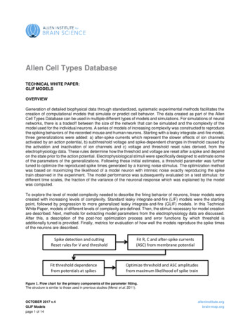
TECHNICAL WHITE PAPERMODEL DEFINITIONSBelow the five different GLIF models are defined in order of increasing level of complexity. Figure 2illustrates the iterations between the state variables in the model equations. Figure 8 shows the progressionof models for two neurons.After-spike currents (ASC)(t)IjI(t)jMembrane potential reset (t)Threshold reset (R)Figure 2. Interactions between state variables for different levels.Leaky Integrate-and-Fire (GLIF1:LIF)The leaky integrate-and-fire (LIF) neuron was a hybrid system characterized by1. An evolution equation for the membrane potential V(t) (which is the only state variable in this case) asa function of the neuron’s capacitance (C), membrane conductance (G), resting potential (E L), and thetime dependent external current (Ie):,2. A reset rule if the membrane potential becomes larger than a thresholdOCTOBER 2017 v.4GLIF Modelspage 2 of 14alleninstitute.orgbrain-map.org
TECHNICAL WHITE PAPERLeaky Integrate-and-Fire with Biologically Defined Reset Rules (GLIF2:LIF-R)LIF-R had evolution equations for two state variables: the membrane potential V(t) and a threshold Θs(t) whichwas updated by spikes and decays back to zero with a temporal constant bs,along with a reset rule if the membrane potential becomes larger than a threshold, which has both a constant(Θ ) and a spike-induced (Θs(t)) component:The update to the spike-dependent component of the threshold is additive with a δΘs added after every spike.The update to the membrane potential has multiplicative coefficient fv, and an additive one δV.Leaky Integrate-and-Fire with After-spike Currents (GLIF3:LIF-ASC)In LIF models, the rapid membrane potential fluctuations due to the fast voltage-activated (i.e. sodium andpotassium) ion channels during a spike were ignored. However, the ion channels activated by a spike couldhave effects over longer time scales. As the sharp membrane potential transitions during an action potentialwere stereotypical, the longer term effects were modeled as additional currents, which had predefined timescales (kj), a multiplicative constant (Rj) which is typically set to 1, and an additive constant (Aj) to each currentfollowing a spike.The update rule, which applies if, changes theLeaky Integrate-and-Fire with Biologically Defined Reset Rules and After-spike Currents (GLIF4:LIF-RASC)Integrating the biological reset rules with the after-spike currents (described above) led to a model defined by:The update rule, which applies ifOCTOBER 2017 v.4GLIF Modelspage 3 of 14,alleninstitute.orgbrain-map.org
TECHNICAL WHITE PAPERLeaky Integrate-and-Fire with Voltage Dependent Threshold, Biologically Defined Reset Rules, andAfter-spike Currents (GLIF5:LIF-R-ASC-AT)Generalized leaky integrate-and-fire (GLIF) neurons were a hybrid system characterized by an evolutionequation for the state variables and a reset rule if a spike occurred. For the LIF-R-ASC-AT, the state variableswere the membrane potential V(t), a set of after-spike currents Ij(t), and a threshold which had spike (Θs) andmembrane potential (Θv) dependent components. It was assumed that these state variables evolved in a linearmanner between spikes:Where C represented the neuron’s capacitance, G the membrane conductance, EL the resting membranepotential, Ie the external current, ki the time constants of the after-spike currents, bs and bv the time constantsof the spike- and voltage-dependent components of the threshold, and a the voltage dependence of thethreshold.A spike was generated ifrules:, and the state variables were updated according to the resetwhere the value immediately after the spike, (t ) was related to the value immediately before the spike (t-) via aset of update parameters: f represented the fraction of the prespike value of a variable which was maintainedafter the spike, and δ represented the values updated by a spike.PARAMETER FITTINGCriteria for Model CreationFor a GLIF model to be created, a base set of stimuli (referred to as “sweeps”) had to pass quality control (QC).For a model of any level to be created, the following sweeps had to pass QC: One subthreshold long square (in order to estimate Maximum Likelihood Based on Internal Noise(MLIN) optimization parameters)OCTOBER 2017 v.4GLIF Modelspage 4 of 14alleninstitute.orgbrain-map.org
TECHNICAL WHITE PAPER One subthreshold short square (to estimate threshold)One suprathreshold short square (to estimate threshold)Two noise 1 (training)Two noise 2 (testing)In addition, for any model requiring reset rules (i.e., LIF-R, LIF-R-ASC or A LIF-R-ASC-AT), a set of triple shortsquare sweeps had to be available. For a description of these stimuli, see the Electrophysiology Overview inthe Documentation tab. The noise stimuli were required for model optimization and testing, while the otherstimuli were needed for parameter extraction as described below. Only sweeps that passed QC were used ineither preprocessing or optimization.Data PreprocessingBefore parameter fitting, there was a preprocessing stage with the primary goal of calculating basic propertiesof the electrophysiological data (such as the resting potential and spike times) and removing the rapidly varyingpotential that occurs during a spike.Resting potential [EL]: The resting potential was defined as the mean resting potential of the noise 1 sweeps ascalculated in the Electrophysiology Overview in the Documentation tab (averaging the pre-stimulusmembrane potential).Spike initiation detection: For a detailed description of how spikes were detected please see the Action PotentialIdentification section of the Electrophysiology Overview in the Documentation tab.Spike cutting: The sections of the voltage traces influenced by the highly non-linear ion fluctuations during theaction potential were not included in the fitting of the subthreshold elements. The duration of the spike, whichwas removed from the trace, was calculated by aligning all of the action potentials of noise 1 to the spikeinitiation (Figure 3). Then a linear dependence was fit between the voltage at spike initiation (prespike voltage)and the voltages at each time point in a window of 1 to 10 ms after spike initiation (postspike voltages). Theduration of the spike was then chosen by considering the linear fit of each prespike and postspike combination.The fit which minimized the residuals was chosen to define the spike duration and voltage reset rules describedbelow (Figure 4).Figure 3. Spike cutting.The action potentials are excluded from model fitting. All spikes from the noise 1 stimuli are aligned. Dots represent spike initiation andtermination found by minimizing the residuals from a linear regression between prespike voltage and postspike voltage in a window 1to 10 ms after spike initiation.Voltage reset rules [V(t )]: When the model spiked, the voltage was reset according to rules that depended onthe model type. In the LIF and LIF-ASC models, the voltage was reset to the resting potential. For the LIF-R,LIF-R-ASC, and LIF-R-ASC-AT models, the postspike voltage was reset via rules extracted from theelectrophysiological traces during the spike cutting calculation described above. The voltage of the model wasOCTOBER 2017 v.4GLIF Modelspage 5 of 14alleninstitute.orgbrain-map.org
TECHNICAL WHITE PAPERreset by Vma slope*Vmb intercept, where Vmb was the voltage of the model before the spike and Vma was thevoltage of the model after the spike (Figure 4). The intercept and slope were calculated via the linear regressionfit to the prespike voltage and postspike voltages explained in the Spike Cutting section above.Figure 4. Reset rules were found by fitting a line between the voltage at spike initiation and the voltage at spike termination.In the LIF-R, LIF-R-ASC, and LIF-R-ASC-AT models, voltage reset is calculated by inserting the model voltage when it reaches thresholdinto the equation defined by the line. Note that the axes on this plot are converted into the model frame of reference by subtracting theresting potential and the prespike non-linearity correction. This correction is applied to the voltage reset rules.Parameter FittingAll fitting (and optimization) requiring noise stimuli were performed on the training noise set (noise 1). Theholdout noise stimuli (noise 2) were reserved for testing to protect against “overfitting”. Descriptions of thespecific fitting calculations follow. Brackets denote the variable notation in the model equation section above.Capacitance [C] and Resistance [1/G]: Capacitance and resistance were calculated via a linear regression ofthe subthreshold noise in the first epoch of noise stimulation within the three-epoch noise sweeps (this stimulusdid not elicit any spikes).After Spike Currents: The membrane potential for a leaky integrate-and-fire neuron with after-spike currentsI j(t) evolved according to the equations outlined first under the LIF-ASC section.For all of the GLIF model levels where after-spike currents were included (LIF-ASC, LIF-R-ASC, and LIF-RASC-AT), after spike currents were modeled using exponential decaying basis functions with an amplitude anda time scale. The time scales and amplitudes were obtained by providing two from a set of five exponentialdecaying basis currents with varied time scales (1/k j) ([3.33, 10, 33.3, 100, 333.33] ms) to a generalized linearmodel (GLM). The GLM was used to calculate the resistance and amplitudes corresponding to each basiscurrent by regressing the sum of the derivative of the voltage, the external current divided by the capacitanceand the leak current (dV/dt Ie/C) against the basis currents and leak term. C, and EL were calculated asmentioned in the above text. The GLM was run with all combinations of two of the five possible time scalesleading to a choice among (5C2 10) pairs of basis currents. The optimal pair of basis currents chosen was theone which resulted in the maximum log-likelihood value.OCTOBER 2017 v.4GLIF Modelspage 6 of 14alleninstitute.orgbrain-map.org
TECHNICAL WHITE PAPERThe basis currents, with their respective amplitudes, were summed together to obtain the total effective afterspike current. To ensure that the GLM estimates were not affected by the very large currents present during aspike, the regression was always performed using the voltage trace with the spikes removed as mentioned inthe Spike Cutting section above.Instantaneous threshold [Ө ]: The model neuron spiked when the voltage of the model crossed the thresholdof the model. An estimate for the instantaneous threshold was the voltage at spike initiation of the lowestamplitude suprathreshold short square. This was an essential parameter, and it was tuned in the post-hocoptimization of every model.Spike component of the threshold [Өs]: The evolution of the threshold of LIF-R, LIF-R-ASC, LIF-R-ASC-ATcontains a “spiking component” of the threshold. This contribution to the threshold represented the effect spikinghad on the threshold of the neuron due to inactivation of voltage-dependent sodium channels. The inactivationcould be interpreted as a rise in the threshold of the neuron, and the movement from the inactive to a closedstate could be modeled as a linear dynamical process. The change in threshold was fit with an exponential, andthe values of its amplitude and time constant were calculated from the triple short square sweep set data (Figure). For each blip in the triple short square data that produced a spike, the voltage at spike initiation (the threshold)was calculated. In this case, the mean of the threshold of the first spike was taken to be the triple short squareinstantaneous threshold. For all spikes that were not “first spikes,” the time since the last spike was calculated(referred to as an ISI). An exponential was then fit to the ISI versus threshold data (Figure 5). The exponentialwas forced to decay to the value of the triple short square instantaneous threshold (the threshold of the firstspike in each short square triple).Figure 5. The spiking component of the threshold is defined by an exponential function fit to the time between spikes and thevoltage at spike initiation of the triple short square data set.Different colors in data represent different sweeps. Black dots denote spike initiation.Subthreshold voltage component of the threshold [ӨV]: LIF-R-ASC-AT contained both a “spiking” component ofthe threshold (see above) and a “subthreshold voltage” component of the threshold. The subthreshold voltagecomponent represented the effect of subthreshold membrane potential on the threshold (e.g., voltagedependence of sodium channel reactivation). The voltage component of the threshold evolved according to thelast equation under LIF-R-ASC-AT.The exact solution for the above evolution equation was then used to obtain initial estimates for the parametersav and bv using a Nelder-Mead simplex optimization.OCTOBER 2017 v.4GLIF Modelspage 7 of 14alleninstitute.orgbrain-map.org
TECHNICAL WHITE PAPERPost-Hoc OptimizationAfter the parameters were extracted from the electrophysiological data as described in the “Iterative ParameterFitting” section, an optimization step was performed. During optimization, the instantaneous threshold wasoptimized using a Nelder-Mead simplex algorithm (Python scipy module scipy.optimize.fmin). Figure 9 showsthe rastergrams of optimized models for two neurons.Forced-spike Model ParadigmDuring optimization, each spike should be fit without erroneous after-spike current history affecting the fitting ofthe subsequent spikes. Therefore, the model was forced to spike at the times the neuron spikes (Figure 6). Themodel continued to run regardless of whether or not the voltage of the model crossed the threshold of the model.The model voltage, threshold, and after-spike amplitudes were forced to reset at the time the neuron spiked.The reset rules were denoted in the GLIF model section above. When a model was run in its normal forwardrunning manner, the prespike values of the voltage, V(t-), threshold, Ө(t-), and AS currents, Ij(t-), were the valuesof the model at the point where the model voltage crossed the model threshold. In the forced spike paradigm,to ensure that the voltage model was reset below the threshold of the model, the prespike voltage was set equalto the prespike threshold, V(t-) Ө(t-) at the time of the neuron spike. Note that this reset only affected LIF-R,LIF-R-ASC, LIF-R-ASC-AT, where the prespike voltage affected the postspike voltage.Figure 6. The MLIN function is evaluated during a forced-spike model paradigm.Translucent colored lines are neuron voltage traces from several repeats of the same stimuli. Solid colored lines are corresponding modeltraces forced to spike at the time of the biological data. Dashed lines are model thresholds. Black tick marks denote non-spike bins specifiedin the MLIN optimization function. Red tick marks denote spike bins. The dots represent the location within the bin where the voltagedifference between the model voltage and model threshold was minimized. Note that the model was run with a resting potential set equalto zero. Here the data traces are shifted so that their resting potential has a mean equal to zero.Objective Function: Maximum Likelihood Based on Internal Noise (MLIN)Similar to a series of previous studies (Paninski, Pillow, Simoncelli, 2004; Dong et al. 2011; Mensi et al. 2012;Pozzorini et al. 2013), the likelihood that the observed spike train was obtained by the model was maximized.However, the exact method of constructing the likelihood was different in that the noise is not tuned but ratheruses a direct estimate of the biological neuron’s internal noise (Maximum Likelihood based on Internal Noise)was used.Because these GLIF models were deterministic, estimating the likelihood required adding a source of noiseexternal to the model. Rather than searching for the parameters of this noise, a parametric description of theinternal noise of each neuron was used (Figure 7). As this internal noise could depend on the membranepotential, and the most relevant potential was near threshold, the variation in membrane potential during thesteady state period of the largest subthreshold square pulse response was characterized.OCTOBER 2017 v.4GLIF Modelspage 8 of 14alleninstitute.orgbrain-map.org
TECHNICAL WHITE PAPERThe probability density of the neuron being at a potential v away from its mean was fit with an exponentiallydecaying function (denoted by “expsymm” in Figure 7):This variation was considered to be additive to the membrane potential of the deterministic neuron. This allowedthe computation of the probability that a neuron with the given noise would produce a spike if the deterministicmodel had a difference between threshold and membrane potential:where c represented the cumulative distribution of the intrinsic noise.The likelihood of the model producing a set of spikes at the times the biological neuron produces them was:However, the model neuron must both produce spikes when the biological neuron does, and not produce spikeswhen the biological neuron does not.The likelihood of a model neuron not producing spikes was not independent for two nearby time points, as theintrinsic noise had a nontrivial autocorrelation. To estimate the likelihood of the model neuron not producingspikes at the times the biological neuron does not produce spikes, one sample for the internal noise was drawnfor each time period of the autocorrelation, and following this time scale a new independent sample was drawn.As such, the inter-spike intervals were binned with bin sizes equal to the autocorrelation (typical autocorrelationstime scales were much smaller than the inter-spike intervals (Figure 7)). The grid times started from a spiketime and advanced by the autocorrelation time scale, ending at a predefined short time (5 ms) before the nextspike. To estimate the likelihood of a neuron not producing a spike within a bin, the minimal difference betweenthreshold and membrane potential within the bin was chosen, which generated the grid differences:The log likelihood of the entire spike train being exactly reproduces wasOCTOBER 2017 v.4GLIF Modelspage 9 of 14alleninstitute.orgbrain-map.org
TECHNICAL WHITE PAPERFigure 7. Parameters of the MLIN objective function were extracted from the data.A distribution of voltages is created from the tailing end of the largest amplitude subthreshold square pulse available (top panel). Thisdistribution is then fit by a symmetrically decaying exponential function denoted as expymm in the plot legends. The width of the non-spikingbins is chosen via a fit of the autocorrelation.SimplexParameters were optimized to minimize MLIN using a simplex algorithm (Nelder-Mead). To optimize normalizedparameters, the parameters of instantaneous threshold and after-spike amplitudes themselves were notoptimized. Instead, the parameters remained at the values provided by the preprocessor, and multiplicativefactors (coefficients) of these parameters were optimized.To ensure that the optimization routine did not return a sub-optimal local minimum, the overall optimization wasrerun three times. Each time the overall optimization was rerun, the coefficients were randomly perturbedbetween an interval of /- 0.3 of their last found optimized value. Within each of the overall reruns, the stabilityof the convergence was confirmed by reinitializing the algorithm (i.e. re-inflating the simplex) three times at theoptimal position in parameter space with a small random perturbation within an interval of /- 0.01 and then rerunning the simplex.Because the voltage dynamics were governed by a first-order linear differential equation, the voltage dynamicswere forward simulated over a single time step using an exact Euler time stepping method. The timestep waschosen to be 0.2 ms. The current that forces the dynamics was averaged across the timestep.MODEL EVALUATION OF SPIKE TIMESAfter all parameters of the model were optimized, the activity of the models was determined using an Eulerexact method. The spike times of the model were evaluated against the spike times of the neuron. Two metricswere used to evaluate how well the models do at reproducing the spike times of the neuron. The first was awidely used correlation-based method published by Schreiber et al. 2003. The second metric (used on thewebsite) was the explained temporal variance described below (Figure 6), which similarly to the reliabilityfocused on how well the temporal dynamic of the response is captured by the model, but it has a value of 0 ifthe model is at chance.OCTOBER 2017 v.4GLIF Modelspage 10 of 14alleninstitute.orgbrain-map.org
TECHNICAL WHITE PAPERA spike train, ST, was represented as a time series of binary numbers. All numbers in the ST were zero unlessa spike occurred: a spike was denoted with a one. Any spike train could be converted into a single trainperistimulus time histogram, stPSTH by convolving a ST with a Gaussian.In the case where there were many repeats of the same stimulus, a peristimulus time histogram (PSTH) couldbe calculated by taking the mean of the stPSTH at each instant in time. If there were n stPSTHi denoted withindex i, where i goes from 1 to n, i 1,2.n, the PSTH was equal to the column mean of the stPSTHi:The variance in spiking output of neurons could be described by the variance of the PSTH. In general, theexplained variance (EV) between any two PSTHs (multiple or single train) would be:The explained temporal variance by the mean across-trials PSTH of the neuron EVD would be an upper limit onhow well the model could perform:where i denotes the ith data stPSTH and n denotes the total number of data sweeps.Since the models here were deterministic, the pairwise explained variance of the data with the model could becalculated by taking the mean of the explained variance between every data stPSTH D and the model PSTHM.where i denotes the ith data stPSTH and n denotes the total number of data sweeps.If the ratio of the pwEV of the model to the data versus the pwEV within the data was equal to 1, the model wasperforming maximally well. The ratio of the pairwise explained variance by the model to that by the multiple trialaverage was reported.OCTOBER 2017 v.4GLIF Modelspage 11 of 14alleninstitute.orgbrain-map.org
TECHNICAL WHITE PAPERFigure 8. Illustration of the five GLIF models from two different transgenic lines (Htr3a 477975366 and Rorb 314822529). The injectedcurrent, Ie(t), is plotted at the top in black. In all panels, the model trans-membrane potential, V(t), is pictured in blue (spike rasters aremarked below), and the threshold, Theta, in dashed green. For models that contain afterspike currents, the total current is in red. The scalebar applies to all panels except to the injected current. GLIF1: Equivalent to the standard LIF model, when V(t) reaches the constantthreshold, a spike is produced. After a short refractory period, V is reset to a constant value. GLIF2: The threshold Өs modestly increasewith each spike, and decays to a constant. When V(t) reaches Theta s, the neuron spikes. After the refractory period, both V and Ө arereset to a value which is dependent on the state of the neuron before the spike. GLIF3: Every action potential induces afterspike currentswhich decay back to zero. The level of induction depends on the state of the neuron before the spike. GLIF4: Here, spike-induced changesin threshold and afterspike currents are combined and reset for all variables which are dependent on the state of the neuron before thespike. GLIF5: The addition of a voltage-dependence to the threshold Ө.OCTOBER 2017 v.4GLIF Modelspage 12 of 14alleninstitute.orgbrain-map.org
TECHNICAL WHITE PAPERFigure 9. Rastergrams of biological data and all optimized model levels for 'hold out' test data for the two example cells: Htr3a477975366 and Rorb 314822529. Injected current shown in black. Black rasters are spikes from recorded neurons to repeated currentinjections. Colored rasters correspond to the five different, deterministic models. The current injection is 3 s long. It is observed that as theGLIF1 and GLIF2 do not have a spike frequency adaptation mechanism, they have trouble reproducing simultaneously the firing patterns atmultiple input amplitudes.PYTHON VERSIONAll code was implemented using python 2.7.8 via Anaconda 2.1.0 (64-bit) compiled with GCC 4.4.7 20120313(Red Hat 4.4.7-1), Numpy version 1.9.0, Scipy version 0.14.0.REFERENCESDong Y, Mihalas S, Russell A, Etienne-Cummings R, Niebur E (2011) Estimating parameters of generalizedintegrate-and-fire neurons from the maximum likelihood of spike trains. Neural Computation 23:2833-2867.Mensi S, Naud R, Pozzorini C, Avermann M, Petersen CC, Gerstner W (2012) Parameter extraction andclassification of three cortical neuron types reveals two distinct adaptation mechanisms. Journal ofNeurophysiology 107:1756-1775.Paninski L, Pillow JW, Simoncelli EP (2004) Maximum likelihood estimation of a stochastic integrate-and-fireneural encoding model. Neural Computation 16:2533-2561.Pozzorini C, Naud R, Mensi S, Gerstner W (2013) Temporal whitening by power-law adaptation in neocorticalneurons. Nature Neuroscience 16:942-948.Schreiber S, Fellous JM, Whitmer D, Tiesinga P, Sejnowski TJ (2003) A new correlation-based measure ofspike timing reliability. Neurocomputing 52-54:925-931.OCTOBER 2017 v.4GLIF Modelspage 13 of 14alleninstitute.orgbrain-map.org
TECHNICAL WHITE PAPERAPPENDIXTable 1. State variables added by each mechanism.ModelSymbolVariableLIFV(t)Membrane potentialASCIj(t)After-spike currentsRӨs(t)Spike-dependent threshold componentTAӨV(t)Voltage-dependent threshold componentThe first level, LIF, contains only the membrane potential V(t). When history dependent reset rules are addedin the second level LIF-R, the sate variables are V(t) and Θs(t). LIF-ASC adds afterspike currents, with the statevariables V(t) and Ij(t), and their combination, LIF-R-ASC has V(t), Θs(t) and Ij(t). Adding the mechanisms whichhas a component of the threshold which is dependent on the membrane potential between spikes, LIF-R-ASCTA leads to the state variables being V(t), Θs(t), ΘV(t) and Ij(t).Table 2. Parameters added by each mechanism.ModelSymbolLIFCCapacitanceV during low amplitude noiseNoLIFGMembrane conductanceSubthreshold V during noiseNoLIFELResting potentialResting V before noiseNoLIF Instantaneous thresholdShort square inputYesRfvVoltage fraction following restAll noise spikesNoR VVoltage addition following restAll noise spikesNoRbsSpike-induced threshold timeconstantTriple short squareNoR Threshold addition following resetTriple short squareNoASCAjAfterspike current amplitudesSubthreshold V during noiseYesASCkjAfterspike current time constantsSubthreshold V during noiseNoT
additionally tuned is provided. Finally, metrics for evaluation of how well the models reproduce the spike times of the neurons are described. Figure 1. Flow chart for the primary components of the parameter fitting. The structure is similar to those used in previous