Transcription
Chapter 5SamplingDistributionsIntroduction to the Practice ofSTATISTICSSEVENTHE DITI ONMoore / McCabe / CraigLecture Presentation Slides
Chapter 5Sampling Distributions5.1 The Sampling Distribution of a Sample Mean5.2 Sampling Distributions for Counts andProportions2
5.1 The Sampling Distributionof a Sample Mean§ Population Distribution vs. Sampling Distribution§ The Mean and Standard Deviation of the Sample Mean§ Sampling Distribution of a Sample Mean§ Central Limit Theorem3
Parameters and StatisticsAs we begin to use sample data to draw conclusions about a widerpopulation, we must be clear about whether a number describes asample or a population.A parameter is a number that describes some characteristic of thepopulation. In statistical practice, the value of a parameter is notknown because we cannot examine the entire population.A statistic is a number that describes some characteristic of asample. The value of a statistic can be computed directly from thesample data. We often use a statistic to estimate an unknownparameter.Remember s and p: statistics come from samples andparameters come from populations.We write µ (the Greek letter mu) for the population mean and σ for thepopulation standard deviation. We write x (x-bar) for the sample mean and sfor the sample standard deviation.4
Statistical EstimationThe process of statistical inference involves using information from asample to draw conclusions about a wider population.Different random samples yield different statistics. We need to be able todescribe the sampling distribution of possible statistic values in order toperform statistical inference.We can think of a statistic as a random variable because it takes numericalvalues that describe the outcomes of the random sampling process.PopulationSampleCollect data from arepresentative Sample.Make an Inferenceabout the Population.5
Sampling VariabilityDifferent random samples yield different statistics. This basic fact is calledsampling variability: the value of a statistic varies in repeated randomsampling.To make sense of sampling variability, we ask, “What would happen if wetook many eSampleSampleSample6
Sampling DistributionsThe law of large numbers assures us that if we measure enoughsubjects, the statistic x-bar will eventually get very close to the unknownparameter µ.If we took every one of the possible samples of a certain size, calculatedthe sample mean for each, and graphed all of those values, we would belooking at a sampling distribution.The population distribution of a variable is the distribution ofvalues of the variable among all individuals in the population.The sampling distribution of a statistic is the distribution ofvalues taken by the statistic in all possible samples of the samesize from the same population.7
Mean and Standard Deviation of aSample MeanMean of a sampling distribution of a sample meanThere is no tendency for a sample mean to fall systematically above orbelow m, even if the distribution of the raw data is skewed. Thus, themean of the sampling distribution is an unbiased estimate of thepopulation mean m.Standard deviation of a sampling distribution of a sample meanThe standard deviation of the sampling distribution measures how muchthe sample mean varies from sample to sample. It is smaller than thestandard deviation of the population by a factor of n.è Averages are less variable than individual observations.8
9
The Sampling Distribution of aSample MeanThe sampling distribution of the sample mean is centered at thepopulation mean µ and is less spread out than the population distribution.Here are the facts.The Sampling Distribution of Sample MeansSuppose that x is the mean of an SRS of size n drawn from a large populationwith mean µ and standard deviation σ . Then :The mean of the sampling distribution of x is µx µ The standard deviation of the sampling distribution of x isσσx nNote : These facts about the mean and standard deviation of x are trueno matter what shape the population distribution has. If individual observations have the N(µ,σ) distribution, then the sample meanof an SRS of size n has the N(µ, σ/ n) distribution regardless of the samplesize n.1010
The Central Limit TheoremMost population distributions are not Normal. What is the shape of thesampling distribution of sample means when the population distributionisn’t Normal?It is a remarkable fact that as the sample size increases, the distributionof sample means changes its shape: it looks less like that of thepopulation and more like a Normal distribution!When the sample is large enough, the distribution of sample means isvery close to Normal, no matter what shape the population distributionhas, as long as the population has a finite standard deviation.Draw an SRS of size n from any population with mean µ and finitestandard deviation σ . The central limit theorem (CLT) says that when nis large, the sampling distribution of the sample mean x is approximatelyNormal:! σ x is approximately N # µ,&"n%11
ExampleBased on service records from the past year, the time (in hours) thata technician requires to complete preventative maintenance on an airconditioner follows the distribution that is strongly right-skewed, andwhose most likely outcomes are close to 0. The mean time is µ 1hour and the standard deviation is σ 1.Your company will service an SRS of 70 air conditioners. You have budgeted 1.1hours per unit. Will this be enough?The central limit theorem states that the sampling distribution of the mean time spentworking on the 70 units is:σ1 0.12μx μ 1n70The sampling distribution of the mean time spent working is approximately N(1, 0.12)because n 70 30. P(x 1.1) P(Z 0.83)1.1 1z 0.83 1 0.7967 0.20330.12σx If you budget 1.1 hours per unit, there is a 20%chance the technicians will not complete thework within the budgeted time.12
13
14
15
A Few More FactsAny linear combination of independent Normalrandom variables is also Normally distributed.More generally, the central limit theorem notesthat the distribution of a sum or average ofmany small random quantities is close toNormal.Finally, the central limit theorem also applies todiscrete random variables.16
5.2 Sampling Distributions forCounts and Proportions§ Binomial Distributions for Sample Counts§ Binomial Distributions in Statistical Sampling§ Finding Binomial Probabilities§ Binomial Mean and Standard Deviation§ Sample Proportions§ Normal Approximation for Counts and Proportions§ Binomial Formula17
The Binomial SettingWhen a random phenomenon is repeated or observed several times, weare often interested in the number of times a particular outcome occurs.Think about tossing a coin n times, where each toss is either a H or T.A binomial setting arises when we perform several independent “trials”, eachwith two possible outcomes: “Success” and “Failure”. The four requirements fora binomial setting are: Binary? The outcomes of each trial can be labeled “Success” or “Failure.” Independent? Trials must be independent; that is, knowing the result of onetrial must not have any effect on the result of any other trial. Number? The number of trials n must be fixed in advance (ie, n is not random). Success? On each trial, the probability p of success must be the same.18
Binomial DistributionConsider tossing a coin n times. Each toss gives either heads or tails.Knowing the outcome of one toss does not change the probability of anoutcome on any other toss. If we define heads as a success, then p is theprobability of a head and is 0.5 on any toss. Thus, we have a binomialsetting.Let the random variable X be the number of heads in those n tosses. Theprobability distribution of X is called a binomial distribution.Binomial DistributionThe count X of successes in a binomial setting has the binomialdistribution with parameters n and p, where n is the number of trialsand p is the probability of a success on any one trial. The possiblevalues of X are the integers from 0 to n. That is, S {0, 1, 2, , n}.Note: Not all counts have binomial distributions; be sure to check theconditions for a binomial setting and make sure you’re being asked to countthe number of successes in a fixed number of trials!19
Binomial Distributions in StatisticalSamplingThe binomial distributions are important in statistics when we want tomake inferences about the proportion p of successes in a population.Suppose 10% of CDs have defective copy-protection schemes that can harmcomputers. A music distributor inspects an SRS of 10 CDs from a shipment of10,000. Let X number of defective CDs.What is P(X 0)? Note: This is not quite a binomial setting. Why?ttThe actual probability isP(no defectives) 9000 8999 89988991 . 0.348510000 9999 99989991Sampling Distribution of a CountChoose an SRS of size n from a population with proportion p of successes.When the populationis much larger than the sample, the count X of successes in the sample has approximately the binomial distribution withparameters n and p.Using the binomial distribution,"10%P(X 0) '(0.10) 0 (0.90)10 0.3487#0&20
Binomial Mean and StandardDeviationMean and Standard Deviation of a Binomial Random VariableIf a count X has a binomial distribution with parameters n and p, the meanand standard deviation of X are:μ X npσ X np (1 p)Note: These formulas work ONLY for binomial distributions.They can’t be used for other distributions!21
Normal Approximation forBinomial DistributionsAs n gets larger, something interesting happens to the shape of abinomial distribution.Normal Approximation for Binomial DistributionsSuppose that X has the binomial distribution with n trials and successprobability p. When n is large, the distribution of X is approximately Normalwith mean and standard deviationµX npσ X np(1 p)As a rule of thumb, we will use the Normal approximation when n is solarge that np 10 and n(1 – p) 10.22
ExampleSample surveys show that fewer people enjoy shopping than in the past. A survey asked anationwide random sample of 2500 adults if they agreed or disagreed that “I like buyingnew clothes, but shopping is often frustrating and time-consuming.” Suppose that exactly60% of all adult U.S. residents would say “Agree” if asked the same question. Let X thenumber in the sample who agree. Estimate the probability that 1520 or more of thesample agree.1) Verify that X is approximately a binomial random variable.B: Success agree, Failure don’t agreeI: Because the population of U.S. adults is greater than 25,000, it is reasonable to assume thesampling without replacement condition is met.N: n 2500 trials of the chance process.S: The probability of selecting an adult who agrees is p 0.60.2) Check the conditions for using a Normal approximation.Since np 2500(0.60) 1500 and n(1 – p) 2500(0.40) 1000 are both at least 10, we may usethe Normal approximation.3) Calculate P(X 1520) using a Normal approximation.μ np 2500(0.60) 1500σ np (1 p) 2500(0.60)(0.40) 24.49z 1520 1500 0.8224.49P(X 1520) P(Z 0.82) 1 0.7939 0.206123
Sampling Distribution of a SampleProportionThere is an important connection between the sample proportion pˆ andthe number of " successes" X in the sample.count of successes in sample Xp̂ size of samplenSampling Distribution of a Sample ProportionChoose an SRS of size n from a population of size N with proportion pof successes. Let pÙ be the sample proportion of successes. Then :The mean of the sampling distribution is p.The standard deviation of the sampling distribution isσ p̂ p(1 p)nFor large n, p̂ has approximately the N( p, p(1 p) / n distribution.As n increases, the sampling distribution becomes approximately Normal.24
Binomial FormulaWe can find a formula for the probability that a binomial random variabletakes any value by adding probabilities for the different ways of gettingexactly that many successes in n observations.The number of ways of arranging k successes among n observationsis given by the binomial coefficient n n! k k!(n k)!for k 0, 1, 2, , n.Note: n! n(n – 1)(n – 2) (3)(2)(1)and 0! 1.25
Binomial ProbabilityThe binomial coefficient counts the number of different ways in whichk successes can be arranged among n trials. The binomial probabilityP(X k) is this count multiplied by the probability of any one specificarrangement of the k successes.Binomial ProbabilityIf X has the binomial distribution with n trials and probability p ofsuccess on each trial, the possible values of X are 0, 1, 2, , n. If kis any one of these values, n kP(X k) p (1 p) n k k 26
ExampleEach child of a particular pair of parents has probability 0.25 of having bloodtype O. Suppose the parents have five children.(a) Find the probability that exactly three of the children have type Oblood.Let X the number of children with type O blood. We know X has a binomial distributionwith n 5 and p 0.25. 5 P(X 3) (0.25) 3 (0.75) 2 10(0.25) 3 (0.75) 2 0.08789 3 (b) Should the parents be surprised if more than three of their childrenhave type O blood?P(X 3) P(X 4) P(X 5) 5 5 41 (0.25) (0.75) (0.25) 5 (0.75) 0 4 5 5(0.25) 4 (0.75)1 1(0.25) 5 (0.75) 0 0.01465 0.00098 0.0156327
Chapter 5Sampling Distributions5.1 The Sampling Distribution of a Sample Mean5.2 Sampling Distributions for Counts andProportions28
STATISTICS EDITION Moore / McCabe / Craig Introduction to the Practice of Chapter 5 Sampling Distributions . 2 Chapter 5 Sampling Distributions 5.1 The Sampling Distribution of a Sample Mean