Transcription
A First Course onTime Series AnalysisExamples with SASChair of Statistics, University of WürzburgAugust 1, 2012
A First Course onTime Series Analysis — Examples with SASby Chair of Statistics, University of Würzburg.Version 2012.August.01Copyright 2012 Michael Falk.EditorsProgramsLayout and Design1234Michael Falk1 , Frank Marohn1 , René Michel2 , DanielHofmann, Maria Macke, Christoph Spachmann, StefanEnglert3Bernward Tewes4 , René Michel2 , Daniel Hofmann,Christoph Spachmann, Stefan Englert3Peter Dinges, Stefan Englert3Institute of Mathematics, University of WürzburgAltran CISInstitute of Medical Biometry and Informatics, University of HeidelbergUniversity Computer Center of the Catholic University of Eichstätt-IngolstadtPermission is granted to copy, distribute and/or modify this document under theterms of the GNU Free Documentation License, Version 1.3 or any later versionpublished by the Free Software Foundation; with no Invariant Sections, no FrontCover Texts, and no Back-Cover Texts. A copy of the license is included in thesection entitled ”GNU Free Documentation License”.SAS and all other SAS Institute Inc. product or service names are registered trademarks or trademarks of SAS Institute Inc. in the USA and other countries. Windowsis a trademark, Microsoft is a registered trademark of the Microsoft Corporation.The authors accept no responsibility for errors in the programs mentioned of theirconsequences.
PrefaceThe analysis of real data by means of statistical methods with the aidof a software package common in industry and administration usuallyis not an integral part of mathematics studies, but it will certainly bepart of a future professional work.The practical need for an investigation of time series data is exemplified by the following plot, which displays the yearly sunspot numbersbetween 1749 and 1924. These data are also known as the Wolf orWölfer (a student of Wolf) Data. For a discussion of these data andfurther literature we refer to Wei and Reilly (1989), Example 6.2.5.Plot 1: Sunspot dataThe present book links up elements from time series analysis with a selection of statistical procedures used in general practice including the
ivstatistical software package SAS (Statistical Analysis System). Consequently this book addresses students of statistics as well as students ofother branches such as economics, demography and engineering, wherelectures on statistics belong to their academic training. But it is alsointended for the practician who, beyond the use of statistical tools, isinterested in their mathematical background. Numerous problems illustrate the applicability of the presented statistical procedures, whereSAS gives the solutions. The programs used are explicitly listed andexplained. No previous experience is expected neither in SAS nor in aspecial computer system so that a short training period is guaranteed.This book is meant for a two semester course (lecture, seminar orpractical training) where the first three chapters can be dealt within the first semester. They provide the principal components of theanalysis of a time series in the time domain. Chapters 4, 5 and 6deal with its analysis in the frequency domain and can be workedthrough in the second term. In order to understand the mathematicalbackground some terms are useful such as convergence in distribution,stochastic convergence, maximum likelihood estimator as well as abasic knowledge of the test theory, so that work on the book can startafter an introductory lecture on stochastics. Each chapter includesexercises. An exhaustive treatment is recommended. Chapter 7 (casestudy) deals with a practical case and demonstrates the presentedmethods. It is possible to use this chapter independent in a seminaror practical training course, if the concepts of time series analysis arealready well understood.Due to the vast field a selection of the subjects was necessary. Chapter 1 contains elements of an exploratory time series analysis, including the fit of models (logistic, Mitscherlich, Gompertz curve)to a series of data, linear filters for seasonal and trend adjustments(difference filters, Census X–11 Program) and exponential filters formonitoring a system. Autocovariances and autocorrelations as wellas variance stabilizing techniques (Box–Cox transformations) are introduced. Chapter 2 provides an account of mathematical modelsof stationary sequences of random variables (white noise, movingaverages, autoregressive processes, ARIMA models, cointegrated sequences, ARCH- and GARCH-processes) together with their mathematical background (existence of stationary processes, covariance
vgenerating function, inverse and causal filters, stationarity condition,Yule–Walker equations, partial autocorrelation). The Box–Jenkinsprogram for the specification of ARMA-models is discussed in detail(AIC, BIC and HQ information criterion). Gaussian processes andmaximum likelihod estimation in Gaussian models are introduced aswell as least squares estimators as a nonparametric alternative. Thediagnostic check includes the Box–Ljung test. Many models of timeseries can be embedded in state-space models, which are introduced inChapter 3. The Kalman filter as a unified prediction technique closesthe analysis of a time series in the time domain. The analysis of aseries of data in the frequency domain starts in Chapter 4 (harmonicwaves, Fourier frequencies, periodogram, Fourier transform and itsinverse). The proof of the fact that the periodogram is the Fouriertransform of the empirical autocovariance function is given. This linksthe analysis in the time domain with the analysis in the frequency domain. Chapter 5 gives an account of the analysis of the spectrum ofthe stationary process (spectral distribution function, spectral density, Herglotz’s theorem). The effects of a linear filter are studied(transfer and power transfer function, low pass and high pass filters,filter design) and the spectral densities of ARMA-processes are computed. Some basic elements of a statistical analysis of a series of datain the frequency domain are provided in Chapter 6. The problem oftesting for a white noise is dealt with (Fisher’s κ-statistic, Bartlett–Kolmogorov–Smirnov test) together with the estimation of the spectral density (periodogram, discrete spectral average estimator, kernelestimator, confidence intervals). Chapter 7 deals with the practicalapplication of the Box–Jenkins Program to a real dataset consisting of7300 discharge measurements from the Donau river at Donauwoerth.For the purpose of studying, the data have been kindly made available to the University of Würzburg. A special thank is dedicated toRudolf Neusiedl. Additionally, the asymptotic normality of the partialand general autocorrelation estimators is proven in this chapter andsome topics discussed earlier are further elaborated (order selection,diagnostic check, forecasting).This book is consecutively subdivided in a statistical part and a SASspecific part. For better clearness the SAS-specific part, includingthe diagrams generated with SAS, is between two horizontal bars,
viseparating it from the rest of the text.12/* This is a sample comment. *//* The first comment in each program will be its name. */345Program code will be set in typewriter-font. SAS keywords like DATA orPROC will be set in bold.6789Also all SAS keywords are written in capital letters. This is notnecessary as SAS code is not case sensitive, but it makes it easier toread the code.101112Extra-long lines will be broken into smaller lines with continuation, marked by an arrow and indentation.(Also, the line-number is missing in this case.)In this area, you will find a step-by-step expla- that SAS cannot be explained as a whole thisnation of the above program. The keywords way. Only the actually used commands will bewill be set in typewriter-font. Please note mentioned.
Contents1 Elements of Exploratory Time Series Analysis11.1 The Additive Model for a Time Series . . . . . . . . .21.2 Linear Filtering of Time Series . . . . . . . . . . . .161.3 Autocovariances and Autocorrelations . . . . . . . .35Exercises . . . . . . . . . . . . . . . . . . . . . . . . . . .412 Models of Time Series472.1 Linear Filters and Stochastic Processes . . . . . . .472.2 Moving Averages and Autoregressive Processes . .612.3 The Box–Jenkins Program . . . . . . . . . . . . . . .99Exercises . . . . . . . . . . . . . . . . . . . . . . . . . . . 1113 State-Space Models1213.1 The State-Space Representation . . . . . . . . . . . 1213.2 The Kalman-Filter . . . . . . . . . . . . . . . . . . . 125Exercises . . . . . . . . . . . . . . . . . . . . . . . . . . . 1324 The Frequency Domain Approach of a Time Series1354.1 Least Squares Approach with Known Frequencies . 1364.2 The Periodogram . . . . . . . . . . . . . . . . . . . . 142Exercises . . . . . . . . . . . . . . . . . . . . . . . . . . . 155
viiiContents5 The Spectrum of a Stationary Process1595.1 Characterizations of Autocovariance Functions . . . 1605.2 Linear Filters and Frequencies . . . . . . . . . . . . 1665.3 Spectral Density of an ARMA-Process . . . . . . . . 175Exercises . . . . . . . . . . . . . . . . . . . . . . . . . . . 1816 Statistical Analysis in the Frequency Domain1876.1 Testing for a White Noise . . . . . . . . . . . . . . . 1876.2 Estimating Spectral Densities . . . . . . . . . . . . . 196Exercises . . . . . . . . . . . . . . . . . . . . . . . . . . . 2167 The Box–Jenkins Program: A Case Study2237.1 Partial Correlation and Levinson–Durbin Recursion . 2247.2 Asymptotic Normality of Partial Autocorrelation Estimator . . . . . . . . . . . . . . . . . . . . . . . . . . 2347.3 Asymptotic Normality of Autocorrelation Estimator . 2597.4 First Examinations . . . . . . . . . . . . . . . . . . . 2727.5 Order Selection . . . . . . . . . . . . . . . . . . . . . 2847.6 Diagnostic Check . . . . . . . . . . . . . . . . . . . . 3117.7 Forecasting . . . . . . . . . . . . . . . . . . . . . . . 324Exercises . . . . . . . . . . . . . . . . . . . . . . . . . . . 335Bibliography337Index341SAS-Index348GNU Free Documentation Licence351
ChapterElements of ExploratoryTime Series AnalysisA time series is a sequence of observations that are arranged accordingto the time of their outcome. The annual crop yield of sugar-beets andtheir price per ton for example is recorded in agriculture. The newspapers’ business sections report daily stock prices, weekly interest rates,monthly rates of unemployment and annual turnovers. Meteorologyrecords hourly wind speeds, daily maximum and minimum temperatures and annual rainfall. Geophysics is continuously observing theshaking or trembling of the earth in order to predict possibly impending earthquakes. An electroencephalogram traces brain waves madeby an electroencephalograph in order to detect a cerebral disease, anelectrocardiogram traces heart waves. The social sciences survey annual death and birth rates, the number of accidents in the home andvarious forms of criminal activities. Parameters in a manufacturingprocess are permanently monitored in order to carry out an on-lineinspection in quality assurance.There are, obviously, numerous reasons to record and to analyze thedata of a time series. Among these is the wish to gain a better understanding of the data generating mechanism, the prediction of futurevalues or the optimal control of a system. The characteristic propertyof a time series is the fact that the data are not generated independently, their dispersion varies in time, they are often governed by atrend and they have cyclic components. Statistical procedures thatsuppose independent and identically distributed data are, therefore,excluded from the analysis of time series. This requires proper methods that are summarized under time series analysis.1
2Elements of Exploratory Time Series Analysis1.1The Additive Model for a Time SeriesThe additive model for a given time series y1 , . . . , yn is the assumption that these data are realizations of random variables Yt that arethemselves sums of four componentsYt Tt Zt St Rt ,t 1, . . . , n.(1.1)where Tt is a (monotone) function of t, called trend , and Zt reflectssome nonrandom long term cyclic influence. Think of the famousbusiness cycle usually consisting of recession, recovery, growth, anddecline. St describes some nonrandom short term cyclic influence likea seasonal component whereas Rt is a random variable grasping allthe deviations from the ideal non-stochastic model yt Tt Zt St .The variables Tt and Zt are often summarized asGt Tt Zt ,(1.2)describing the long term behavior of the time series. We suppose inthe following that the expectation E(Rt ) of the error variable existsand equals zero, reflecting the assumption that the random deviationsabove or below the nonrandom model balance each other on the average. Note that E(Rt ) 0 can always be achieved by appropriatelymodifying one or more of the nonrandom components.Example 1.1.1. (Unemployed1 Data). The following data yt , t 1, . . . , 51, are the monthly numbers of unemployed workers in thebuilding trade in Germany from July 1975 to September 4735748320602198441811991612435087309
1.1 The Additive Model for a Time 215499Listing 1.1.1: Unemployed1 Data.123/* unemployed1 listing.sas */TITLE1 ’Listing’;TITLE2 ’Unemployed1 Data’;45678/* Read in the data (Data-step) */DATA data1;INFILE ’c:\data\unemployed1.txt’;INPUT month t unemplyd;3
4Elements of Exploratory Time Series Analysis9101112/* Print the data (Proc-step) */PROC PRINT DATA data1 NOOBS;RUN;QUIT;This program consists of two main parts, aDATA and a PROC step.The DATA step started with the DATA statementcreates a temporary dataset named data1.The purpose of INFILE is to link the DATA stepto a raw dataset outside the program. The pathname of this dataset depends on the operating system; we will use the syntax of MS-DOS,which is most commonly known. INPUT tellsSAS how to read the data. Three variables aredefined here, where the first one contains character values. This is determined by the signbehind the variable name. For each variableone value per line is read from the source intothe computer’s memory.ThestatementPROC procedurenameDATA filename; invokes a procedure thatis linked to the data from filename. Withoutthe option DATA filename the most recentlycreated file is used.The PRINT procedure lists the data; it comeswith numerous options that allow control of thevariables to be printed out, ’dress up’ of the display etc. The SAS internal observation number(OBS) is printed by default, NOOBS suppressesthe column of observation numbers on eachline of output. An optional VAR statement determines the order (from left to right) in which variables are displayed. If not specified (like here),all variables in the data set will be printed in theorder they were defined to SAS. Entering RUN;at any point of the program tells SAS that a unitof work (DATA step or PROC) ended. SAS thenstops reading the program and begins to execute the unit. The QUIT; statement at the endterminates the processing of SAS.A line starting with an asterisk * and endingwith a semicolon ; is ignored. These commentstatements may occur at any point of the program except within raw data or another statement.The TITLE statement generates a title. Itsprinting is actually suppressed here and in thefollowing.The following plot of the Unemployed1 Data shows a seasonal component and a downward trend. The period from July 1975 to September1979 might be too short to indicate a possibly underlying long termbusiness cycle.
1.1 The Additive Model for a Time SeriesPlot 1.1.2: Unemployed1 Data.123/* unemployed1 plot.sas */TITLE1 ’Plot’;TITLE2 ’Unemployed1 Data’;45678/* Read in the data */DATA data1;INFILE ’c:\data\unemployed1.txt’;INPUT month t unemplyd;910111213/* Graphical Options */AXIS1 LABEL (ANGLE 90 ’unemployed’);AXIS2 LABEL (’t’);SYMBOL1 V DOT C GREEN I JOIN H 0.4 W 1;1415161718/* Plot the data */PROC GPLOT DATA data1;PLOT unemplyd*t / VAXIS AXIS1 HAXIS AXIS2;RUN; QUIT;Variables can be plotted by using the GPLOTprocedure, where the graphical output is controlled by numerous options.The AXIS statements with the LABEL optionscontrol labelling of the vertical and horizontalaxes. ANGLE 90 causes a rotation of the labelof 90 so that it parallels the (vertical) axis inthis example.The SYMBOL statement defines the mannerin which the data are displayed.V DOTC GREEN I JOIN H 0.4 W 1 tell SAS toplot green dots of height 0.4 and to jointhem with a line of width 1.The PLOTstatement in the GPLOT procedure is ofthe form PLOT y-variable*x-variable /options;, where the options here define thehorizontal and the vertical axes.5
6Elements of Exploratory Time Series AnalysisModels with a Nonlinear TrendIn the additive model Yt Tt Rt , where the nonstochastic componentis only the trend Tt reflecting the growth of a system, and assumingE(Rt ) 0, we haveE(Yt ) Tt : f (t).A common assumption is that the function f depends on several (unknown) parameters β1 , . . . , βp , i.e.,f (t) f (t; β1 , . . . , βp ).(1.3)However, the type of the function f is known. The unknown parameters β1 , . . . ,βp are then to be estimated from the set of realizationsyt of the random variables Yt . A common approach is a least squaresestimate β̂1 , . . . , β̂p satisfyingX 2 2X yt f (t; β̂1 , . . . , β̂p ) minyt f (t; β1 , . . . , βp ) , (1.4)β1 ,.,βpttwhose computation, if it exists at all, is a numerical problem. Thevalue ŷt : f (t; β̂1 , . . . , β̂p ) can serve as a prediction of a future yt .The observed differences yt ŷt are called residuals. They containinformation about the goodness of the fit of our model to the data.In the following we list several popular examples of trend functions.The Logistic FunctionThe functionflog (t) : flog (t; β1 , β2 , β3 ) : β3,1 β2 exp( β1 t)t R,with β1 , β2 , β3 R \ {0} is the widely used logistic function.(1.5)
1.1 The Additive Model for a Time SeriesPlot 1.1.3: The logistic function flog with different values of β1 , β2 , β312/* logistic.sas */TITLE1 ’Plots of the Logistic Function’;3456789101112131415/* Generate the data for different logistic functions */DATA data1;beta3 1;DO beta1 0.5, 1;DO beta2 0.1, 1;DO t -10 TO 10 BY 0.5;s COMPRESS(’(’ beta1 ’,’ beta2 ’,’ beta3 ’)’);f log beta3/(1 21222324/* Graphical Options */SYMBOL1 C GREEN V NONE I JOIN L 1;SYMBOL2 C GREEN V NONE I JOIN L 2;SYMBOL3 C GREEN V NONE I JOIN L 3;SYMBOL4 C GREEN V NONE I JOIN L 33;AXIS1 LABEL (H 2 ’f’ H 1 ’log’ H 2 ’(t)’);AXIS2 LABEL (’t’);LEGEND1 LABEL (F CGREEK H 2 ’(b’ H 1 ’1’ H 2 ’, b’ H 1 ’2’ H 2 ’,b’ H, 1 ’3’ H 2 ’) ’);2526/* Plot the functions */7
8Elements of Exploratory Time Series Analysis272829PROC GPLOT DATA data1;PLOT f log*t s / VAXIS AXIS1 HAXIS AXIS2 LEGEND LEGEND1;RUN; QUIT;A function is plotted by computing its values atnumerous grid points and then joining them.The computation is done in the DATA step,where the data file data1 is generated. It contains the values of f log, computed at the gridt 10, 9.5, . . . , 10 and indexed by the vector s of the different choices of parameters.This is done by nested DO loops. The operator merges two strings and COMPRESS removes the empty space in the string. OUTPUTthen stores the values of interest of f log, tand s (and the other variables) in the data setdata1.The four functions are plotted by the GPLOTprocedure by adding s in the PLOT statement.This also automatically generates a legend,which is customized by the LEGEND1 statement. Here the label is modified by using agreek font (F CGREEK) and generating smallerletters of height 1 for the indices, while assuming a normal height of 2 (H 1 and H 2). Thelast feature is also used in the axis statement.For each value of s SAS takes a new SYMBOLstatement. They generate lines of different linetypes (L 1, 2, 3, 33).We obviously have limt flog (t) β3 , if β1 0. The value β3 oftenresembles the maximum impregnation or growth of a system. Notethat11 β2 exp( β1 t) flog (t)β31 exp( β1 )1 β2 exp( β1 (t 1)) exp( β1 )β3β31 exp( β1 )1 exp( β1 )β3flog (t 1)b a .(1.6)flog (t 1) This means that there is a linear relationship among 1/flog (t). Thiscan serve as a basis for estimating the parameters β1 , β2 , β3 by anappropriate linear least squares approach, see Exercises 1.2 and 1.3.In the following example we fit the logistic trend model (1.5) to thepopulation growth of the area of North Rhine-Westphalia (NRW),which is a federal state of Germany.Example 1.1.2. (Population1 Data). Table 1.1.1 shows the population sizes yt in millions of the area of North-Rhine-Westphalia in
1.1 The Additive Model for a Time Series95 years steps from 1935 to 1980 as well as their predicted values ŷt ,obtained from a least squares estimation as described in (1.4) for alogistic model.Yeart Population sizes yt Predicted values ŷt(in millions)(in millions)1935 11940 21945 31950 41955 51960 61965 71970 81975 91980 .88116.54817.15817.710Table 1.1.1: Population1 DataAs a prediction of the population size at time t we obtain in the logisticmodelŷt : β̂31 β̂2 exp( β̂1 t)21.5016 1 1.1436 exp( 0.1675 t)with the estimated saturation size β̂3 21.5016. The following plotshows the data and the fitted logistic curve.
10Elements of Exploratory Time Series AnalysisPlot 1.1.4: NRW population sizes and fitted logistic function.123/* population1.sas */TITLE1 ’Population sizes and logistic fit’;TITLE2 ’Population1 Data’;45678/* Read in the data */DATA data1;INFILE ’c:\data\population1.txt’;INPUT year t pop;91011121314/* Compute parameters for fitted logistic function */PROC NLIN DATA data1 OUTEST estimate;MODEL pop beta3/(1 beta2*EXP(-beta1*t));PARAMETERS beta1 1 beta2 1 beta3 20;RUN;1516171819202122/* Generate fitted logistic function */DATA data2;SET estimate(WHERE ( TYPE ’FINAL’));DO t1 0 TO 11 BY 0.2;f log beta3/(1 beta2*EXP(-beta1*t1));OUTPUT;END;2324252627/* Merge data sets */DATA data3;MERGE data1 data2;
1.1 The Additive Model for a Time Series282930313211/* Graphical options */AXIS1 LABEL (ANGLE 90 ’population in millions’);AXIS2 LABEL (’t’);SYMBOL1 V DOT C GREEN I NONE;SYMBOL2 V NONE C GREEN I JOIN W 1;3334353637/* Plot data with fitted function */PROC GPLOT DATA data3;PLOT pop*t 1 f log*t1 2 / OVERLAY VAXIS AXIS1 HAXIS AXIS2;RUN; QUIT;The procedure NLIN fits nonlinear regressionmodels by least squares. The OUTEST optionnames the data set to contain the parameterestimates produced by NLIN. The MODEL statement defines the prediction equation by declaring the dependent variable and defining an expression that evaluates predicted values. APARAMETERS statement must follow the PROCNLIN statement. Each parameter value expression specifies the starting values of the pa-rameter. Using the final estimates of PROCNLIN by the SET statement in combination withthe WHERE data set option, the second datastep generates the fitted logistic function values. The options in the GPLOT statement causethe data points and the predicted function to beshown in one plot, after they were stored together in a new data set data3 merging data1and data2 with the MERGE statement.The Mitscherlich FunctionThe Mitscherlich function is typically used for modelling the longterm growth of a system:fM (t) : fM (t; β1 , β2 , β3 ) : β1 β2 exp(β3 t),t 0,(1.7)where β1 , β2 R and β3 0. Since β3 is negative we have theasymptotic behavior limt fM (t) β1 and thus the parameter β1 isthe saturation value of the system. The (initial) value of the systemat the time t 0 is fM (0) β1 β2 .The Gompertz CurveA further quite common function for modelling the increase or decrease of a system is the Gompertz curvefG (t) : fG (t; β1 , β2 , β3 ) : exp(β1 β2 β3t ),where β1 , β2 R and β3 (0, 1).t 0,(1.8)
12Elements of Exploratory Time Series AnalysisPlot 1.1.5: Gompertz curves with different parameters.12/* gompertz.sas */TITLE1 ’Gompertz curves’;3456789101112131415/* Generate the data for different Gompertz functions */DATA data1;beta1 1;DO beta2 -1, 1;DO beta3 0.05, 0.5;DO t 0 TO 4 BY 0.05;s COMPRESS(’(’ beta1 ’,’ beta2 ’,’ beta3 ’)’);f g EXP(beta1 3/* Graphical Options */SYMBOL1 C GREEN V NONE I JOIN L 1;SYMBOL2 C GREEN V NONE I JOIN L 2;SYMBOL3 C GREEN V NONE I JOIN L 3;SYMBOL4 C GREEN V NONE I JOIN L 33;AXIS1 LABEL (H 2 ’f’ H 1 ’G’ H 2 ’(t)’);AXIS2 LABEL (’t’);
1.1 The Additive Model for a Time Series2413LEGEND1 LABEL (F CGREEK H 2 ’(b’ H 1 ’1’ H 2 ’,b’ H 1 ’2’ H 2 ’,b’ H 1, ’3’ H 2 ’) ’);2526272829/*Plot the functions */PROC GPLOT DATA data1;PLOT f g*t s / VAXIS AXIS1 HAXIS AXIS2 LEGEND LEGEND1;RUN; QUIT;We obviously havelog(fG (t)) β1 β2 β3t β1 β2 exp(log(β3 )t),and thus log(fG ) is a Mitscherlich function with parameters β1 , β2 andlog(β3 ). The saturation size obviously is exp(β1 ).The Allometric FunctionThe allometric functionfa (t) : fa (t; β1 , β2 ) β2 tβ1 ,t 0,(1.9)with β1 R, β2 0, is a common trend function in biometry andeconomics. It can be viewed as a particular Cobb–Douglas function,which is a popular econometric model to describe the output producedby a system depending on an input. Sincelog(fa (t)) log(β2 ) β1 log(t),t 0,is a linear function of log(t), with slope β1 and intercept log(β2 ), wecan assume a linear regression model for the logarithmic data log(yt )log(yt ) log(β2 ) β1 log(t) εt ,t 1,where εt are the error variables.Example 1.1.3. (Income Data). Table 1.1.2 shows the (accumulated)annual average increases of gross and net incomes in thousands DM(deutsche mark) in Germany, starting in 1960.
14Elements of Exploratory Time Series AnalysisYeart Gross income xt Net income yt1960 01961 11962 21963 31964 41965 51966 61967 71968 81969 91970 .482Table 1.1.2: Income Data.We assume that the increase of the net income yt is an allometricfunction of the time t and obtainlog(yt ) log(β2 ) β1 log(t) εt .(1.10)The least squares estimates of β1 and log(β2 ) in the above linear regression model are (see, for example Falk et al., 2002, Theorem 3.2.2)P10(log(t) log(t))(log(yt ) log(y))β̂1 t 1 P10 1.019,2(log(t) log(t))t 1P10P1011where log(t) : 10t 1 log(t) 1.5104, log(y) : 10t 1 log(yt ) 0.7849, and hence\2 ) log(y) β̂1 log(t) 0.7549log(βWe estimate β2 therefore byβ̂2 exp( 0.7549) 0.4700.The predicted value ŷt corresponds to the time tŷt 0.47t1.019 .(1.11)
1.1 The Additive Model for a Time Seriestyt 017-0.1583-0.2526-0.09420.5662Table 1.1.3: Residuals of Income Data.Table 1.1.3 lists the residuals yt ŷt by which one can judge thegoodness of fit of the model (1.11).A popular measure for assessing the fit is the squared multiple correlation coefficient or R2 -valuePn(yt ŷt )2R2 : 1 Pt 1(1.12)n2(y ȳ)tt 1Pwhere ȳ : n 1 nt 1 yt is the average of the observations yt (cf Falket al., 2002, Section 3.3). In the linear regression model with ŷt basedon the least squares estimates of the parameters, R2 is necessarilyPnbetween zero and one with the implications R2 1 iff1t 1 (yt 22ŷt ) 0 (see Exercise 1.4). A value of R close to 1 is in favor ofthe fitted model. The model (1.10) has R2 equal to 0.9934, whereas(1.11) has R2 0.9789. Note, however, that the initial model (1.9) isnot linear and β̂2 is not the least squares estimates, in which case R2is no longer necessarily between zero and one and has therefore to beviewed with care as a crude measure of fit.The annual average gross income in 1960 was 6148 DM and the corresponding net income was 5178 DM. The actual average gross andnet incomes were therefore x̃t : xt 6.148 and ỹt : yt 5.178 with1if and only if15
16Elements of Exploratory Time Series Analysisthe estimated model based on the above predicted values ŷtỹˆt ŷt 5.178 0.47t1.019 5.178.Note that the residuals ỹt ỹˆt yt ŷt are not influenced by addingthe constant 5.178 to yt . The above models might help judging theaverage tax payer’s situation between 1960 and 1970 and to predicthis future one. It is apparent from the residuals in Table 1.1.3 thatthe net income yt is an almost perfect multiple of t for t between 1and 9, whereas the large increase y10 in 1970 seems to be an outlier.Actually, in 1969 the German government had changed and in 1970 along strike in Germany caused an enormous increase in the income ofcivil servants.1.2Linear Filtering of Time SeriesIn the following we consider the additive model (1.1) and assume thatthere is no long term cyclic component. Nevertheless, we allow atrend, in which case the smooth nonrandom component Gt equals thetrend function Tt . Our model is, therefore, the decompositionYt Tt St Rt ,t 1, 2, . . .(1.13)with E(Rt ) 0. Given realizations yt , t 1, 2, . . . , n, of this timeseries, the aim of this section is the derivation of estimators T̂t , Ŝtof the nonrandom functions Tt and St and to
vi separating it from the rest of the text. 1 /* This is a sample comment. 2 /* The first comment in each program will be its name. 3 4 Program code will be set in typewriter-font. SAS keywords like DATA or 5 PROC will be set in bold. 6 7 Also all SAS keywords are written in capital letters. This is not 8 necessary as