Transcription
B RIEFINGS IN BIOINF ORMATICS . VOL 7. NO 1. 86 112doi:10.1093/bib/bbk007Machine learning in bioinformaticsPedro Larran‹aga, Borja Calvo, Roberto Santana, Concha Bielza, Josu Galdiano, In‹aki Inza, Jose A. Lozano,Rube n Arman‹anzas, Guzma n Santafe , Aritz Pe rez and Victor RoblesSubmitted: 29th July 2005; Received (in revised form): 21st October 2005AbstractThis article reviews machine learning methods for bioinformatics. It presents modelling methods, such as supervisedclassification, clustering and probabilistic graphical models for knowledge discovery, as well as deterministic andstochastic heuristics for optimization. Applications in genomics, proteomics, systems biology, evolution and textmining are also shown.Keywords: machine learning; bioinformatics; supervised classification; clustering; probabilistic graphical models; optimisation;heuristic; genomics; proteomics; microarray; system biology; evolution; text miningCorresponding author. Pedro Larrañaga, Intelligent Systems Group, Department of Computer Science and Artificial Intelligence,University of the Basque Country, Paseo Manuel de Lardizabal, 1, 20018 San Sebastian, Spain. Tel: þ34943018045; Fax:þ34934015590; E-mail: pedro.larranaga@ehu.esPedro Larran‹aga is Professor of Computer Science and Artificial Intelligence at the University of the Basque Country. He receivedMS degree in mathematics from the University of Valladolid in 1981, and PhD in computer science from the University of the BasqueCountry in 1995. He has published over 40 refereed journal papers. His main research interests are in the areas of evolutionarycomputation, machine learning, probabilistic graphical models and bioinformatics.Borja Calvo received MS in Biochemistry in 1999 and Bachelor degree in Computer Science in 2004, both from the University ofthe Basque Country. Currently he is a PhD student at the University of the Basque Country and a member of the Intelligent SystemsGroup. His research interests include machine learning methods applied to bioinformatics.Roberto Santana received PhD in Mathematics from the University of Havana in 2005. At present, he is at the University of theBasque Country as a member of the Intelligent Systems Group. His research interests include estimation of distribution algorithms andbioinformatics.Concha Bielza received her MS degree in Mathematics in 1989 from Complutense University, Madrid, and PhD in ComputerScience in 1996 from Technical University of Madrid, Madrid. She is an Associate Professor of Statistics and Operation Research in theSchool of Computer Science at Madrid Technical University. Her research interests are primarily in the areas of probabilistic graphicalmodels, decision analysis, metaheuristics for optimization, data mining, classification models and real applications. Her research hasappeared in journals like Management Science, Computers and Operations Research, Statistics and Computing, Naval ResearchLogistics, Journal of the Operational Research Society and as chapters of many books.Josu Galdiano is currently doing his MS in Computer Science at the University of the Basque Country. His research interests includemachine learning methods applied to bioinformatics.In‹aki Inza is a Lecturer at the Intelligent Systems Group of the University of the Basque Country. His research interests include datamining and search heuristics in general, with special focus on probabilistic graphical models and bioinformatic applications.Jose A. Lozano received his BS degrees in Mathematics and Computer Science and the PhD degree from the University of the BasqueCountry, Spain in 1991, 1992 and 1998, respectively. Since 1999, he has been an Associate Professor of Computer Science at theUniversity of the Basque Country. He has edited three books and has published over 25 refereed journal papers. His main researchinterests are evolutionary computation, machine learning, probabilistic graphical models and bioinformatics.Rube n Arman‹anzas received his MS in Computer Science from the University of the Basque Country in 2004. At present, he is a PhDstudent and member of the Intelligent Systems Group. His research interests include feature selection, computational biology and bioinformatics.Guzma n Santafe received his MS in Computer Science from the University of the Basque Country in 2002. At present, he is a PhD studentat the University of the Basque Country and member of the Intelligent Systems Group. His research interests include machine learningtechniques applied to bioinformatics.Aritz Pe rez received her Computer Science degree from the University of the Basque Country. He is currently pursuing PhD in ComputerScience in the Department of Computer Science and Artificial Intelligence. His research interests include machine learning, data mining andbioinformatics. Currently, he is working on supervised classification using Bayesian networks, variable selection and density estimation, focusedfor continuous domains.Victor Robles received the MS degree in Computer Engineering and PhD from the Universidad Politécnica de Madrid, in 1998 and 2003,respectively. During 2004, he was a postdoctoral researcher at Harvard Medical School. He is currently an associate professor in the Departmentof Computer Systems Architecture and Technology at the Universidad Politécnica de Madrid. His research interests include bioinformatics, datamining and optimization. Dr Robles has been involved in the organization of several workshops and publications, as well as in several books onproceedings.ß The Author 2006. Published by Oxford University Press. For Permissions, please email: journals.permissions@oxfordjournals.org
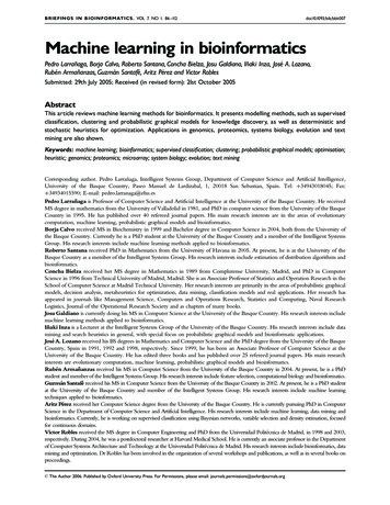
Machine learning in bioinformatics87INTRODUCTIONThe exponential growth of the amount of biologicaldata available raises two problems: on one hand,efficient information storage and managementand, on the other hand, the extraction of usefulinformation from these data. The second problem isone of the main challenges in computational biology,which requires the development of tools andmethods capable of transforming all these heterogeneous data into biological knowledge about theunderlying mechanism. These tools and methodsshould allow us to go beyond a mere description ofthe data and provide knowledge in the form oftestable models. By this simplifying abstraction thatconstitutes a model, we will be able to obtainpredictions of the system.There are several biological domains wheremachine learning techniques are applied for knowledge extraction from data. Figure 1 showsa scheme of the main biological problems wherecomputational methods are being applied. We haveclassified these problems into six different domains:genomics, proteomics, microarrays, systems biology,evolution and text mining. The category named‘other applications’ groups together the remainingproblems. These categories should be understoodin a very general way, especially genomics andproteomics, which in this review are consideredas the study of nucleotide chains and proteins,respectively.Genomics is one of the most important domains inbioinformatics. The number of sequences availableis increasing exponentially, as shown in Figure 2.These data need to be processed in order to obtainuseful information. As a first step, from genomesequences, we can extract the location and structureof the genes [1]. More recently, the identification ofregulatory elements [2–4] and non-coding RNAgenes [5] is also being tackled from a computationalpoint of view. Sequence information is also usedfor gene function and RNA secondary structureprediction.If the genes contain the information, proteins arethe workers that transform this information into life.Proteins play a very important role in the life process,and their three-dimensional (3D) structure is a keyfeature in their functionality. In the proteomic domain,the main application of computational methods isprotein structure prediction. Proteins are verycomplex macromolecules with thousands of atomsand bounds. Hence, the number of possiblestructures is huge. This makes protein structureprediction a very complicated combinatorialproblem where optimization techniques arerequired. In proteomics, as in the case of genomics,machine learning techniques are applied for proteinfunction prediction.Another interesting application of computationalmethods in biology is the management of complexexperimental data. Microarray essays are the bestknown (but not the only) domain where this kindof data is collected. Complex experimental dataraise two different problems. First, data need to bepre-processed, i.e. modified to be suitably used bymachine learning algorithms. Second, the analysis ofthe data, which depends on what we are looking for.In the case of microarray data, the most typicalapplications are expression pattern identification,classification and genetic network induction.Systems biology is another domain where biologyand machine learning work together. It is verycomplex to model the life processes that take placeinside the cell. Thus, computational techniquesare extremely helpful when modelling biologicalnetworks [6], especially genetic networks, signaltransduction networks and metabolic pathways.Evolution and, especially phylogenetic treereconstruction also take advantage of machinelearning techniques. Phylogenetic trees are schematic representations of organisms’ evolution.Traditionally, they were constructed according todifferent features (morphological features, metabolicfeatures, etc.) but, nowadays, with the great amountof genome sequences available, phylogenetic treeconstruction algorithms are based on the comparisonbetween different genomes [7]. This comparisonis made by means of multiple sequencealignment, where optimization techniques are veryuseful.A side effect of the application of computationaltechniques to the increasing amount of data is anincrease in available publications. This provides anew source of valuable information, where textmining techniques are required for the knowledgeextraction. Thus, text mining is becoming more andmore interesting in computational biology, and it isbeing applied in functional annotation, cellularlocation prediction and protein interaction analysis[8]. A review of the application of text miningtechniques in biology and biomedicine can be foundin Ananiadou and McNaught [9].
88Larran‹aga et al.Figure 1: Classification of the topics where machine learning methods are applied.In addition to all these applications, computational techniques are used to solve other problems,such as efficient primer design for PCR, biologicalimage analysis and backtranslation of proteins (whichis, given the degeneration of the genetic code,a complex combinatorial problem).Machine learning consists in programmingcomputers to optimize a performance criterionby using example data or past experience. Theoptimized criterion can be the accuracy provided bya predictive model—in a modelling problem—,and the value of a fitness or evaluation function—inan optimization problem.In a modelling problem, the ‘learning’ term refers torunning a computer program to induce a model byusing training data or past experience. Machinelearning uses statistical theory when buildingcomputational models since the objective is tomake inferences from a sample. The two mainsteps in this process are to induce the model byprocessing the huge amount of data and to representthe model and making inferences efficiently. It mustbe noticed that the efficiency of the learning andinference algorithms, as well as their space andtime complexity and their transparency and interpretability, can be as important as their predictiveaccuracy. The process of transforming data intoknowledge is both iterative and interactive. Theiterative phase consists of several steps. In the firststep, we need to integrate and merge the differentsources of information into only one format. Byusing data warehouse techniques, the detection andresolution of outliers and inconsistencies are solved.In the second step, it is necessary to select, clean andtransform the data. To carry out this step, we need toeliminate or correct the uncorrected data, as well as
Machine learning in bioinformaticsFigure 2: Evolution of the GenBank database size.decide the strategy to impute missing data. This stepalso selects the relevant and non-redundant variables;this selection could also be done with respect to theinstances. In the third step, called data mining, wetake the objectives of the study into account in orderto choose the most appropriate analysis for the data.In this step, the type of paradigm for supervised orunsupervised classification should be selected and themodel will be induced from the data. Once themodel is obtained, it should be evaluated andinterpreted—both from statistical and biologicalpoints of view—and, if necessary, we should returnto the previous steps for a new iteration. Thisincludes the solution of conflicts with the currentknowledge in the domain. The model satisfactorilychecked—and the new knowledge discovered—arethen used to solve the problem.Optimization problems can be posed as the task offinding an optimal solution in a space of multiple(sometimes exponentially sized) possible solutions.The choice of the optimization method to be usedis crucial for the problem solution. Optimizationapproaches to biological problems can be classified,according to the type of solutions found, into exactand approximate methods. Exact methods output theoptimal solutions when convergence is achieved.However, they do not necessarily converge for every89instance. Approximate algorithms always output acandidate solution, but it is not guaranteed to be theoptimal one.Optimization is also a fundamental task whenmodelling from data. In fact, the process of learningfrom data can be regarded as searching for the modelthat gives the data the best fitting. In this search, inthe space of models any type of heuristic can be used.Therefore, optimization methods can also be seen asan ingredient at modelling.There are several reference books on machinelearning topics [10–15]. Recently, some interestingbooks intersecting machine learning and bioinformatics domains have been published [7, 16–27].Special issues in journals [28–30] have also beenpublished covering machine learning topics inbioinformatics.The goal of this article is to serve as an insightfulcategorization and classification of the machinelearning methods in bioinformatics including a listingof their applications and providing a context forreaders new to the field. Due to space restrictions,this article must not be considered a detaileddiscussion of the different methods in modellingand optimization.This article is organized as follows. ‘Supervisedclassification’ section presents the supervised classification problem, techniques for assessing and comparing classification algorithms, feature subset selectionand several classification paradigms. ‘Clustering’section shows different types of clustering—partitionclustering, hierarchical clustering and clusteringbased on mixture models—as well as validationtechniques. ‘Probabilistic graphical models’ sectionfocuses on probabilistic graphical models, a paradigmable to produce supervised and unsupervised models,and to discover knowledge in molecular biologydomains. ‘Optimization’ section shows heuristicoptimization methods that have been proposed inbioinformatics to solve some hard computationalproblems. In all the previous sections, pointers tobioinformatics literature are provided. Final sectionexplains the conclusions of this revision on machinelearning methods in bioinformatics.SUPERVISED CLASSIFICATIONIntroductionIn a classification problem, we have a set of elementsdivided into classes. Given an element (or instance)of the set, a class is assigned according to some of the
90Larran‹aga et al.element’s features and a set of classification rules.In many real-life situations, this set of rules is notknown, and the only information available is a set oflabelled examples (i.e. a set of instances associatedwith a class). Supervised classification paradigms arealgorithms that induce the classification rules fromthe data.As an example, we will see a possible way totackle splice site prediction as a supervised classification problem. The instances to be classified will beDNA sequences of a given size (for example, 22 basepairs, 10 upstream and 10 downstream the 2 bp splicesite). The attributes of a given instance will bethe nucleotide at each position in the sequence.In the example, we will assume that we are lookingfor donor sites, so the possible values for the class willbe true donor site or false donor site. As we areapproaching the problem as supervised classification,we need a set of labelled examples, i.e. a set ofsequences of true and false donor sites along withtheir label. At this point, we can use this training setto build up a classifier. Once the classifier has beentrained, we can use it to label new sequences, usingthe nucleotide present at each position as an inputto the classifier and getting the assigned label (true orfalse donor site) as an output.In two-group supervised classification, there is afeature vector X 2 n whose components are calledpredictor variables and a label or class variable C 2 {0, 1}.Hence, the task is to induce classifiers from trainingdata, which consists of a set of N independentobservationsDN ¼ fðxð1Þ ; cð1Þ Þ; . . . ;ðxðNÞ ; cðNÞ Þgdrawn from the joint probability distribution p(x, c)as shown in Table 1. The classification model willbe used to assign labels to new instances according tothe value of its predictor variables.Assessing and comparingclassification algorithmsError rate and ROC curveWhen a 0/1 loss is used, all errors are equallybad, and our error calculations are based on theconfusion matrix (Table 2). In this case, we candefine the error rate as ( FN þ FP )/N, whereN ¼ TP þ FP þ TN þ FN is the totalnumber of instances in the validation set.To fine-tune a classifier, another approach is todraw the receiver operating characteristics (ROCs) curve[31], which shows hit rate versus false alarm rate,namely, 1-specificity ¼ FP /( FP þ TN ) versussensitivity ¼ TP /( TP þ FN ), and has a formTable 1: Raw data in a supervised classificationproblem(x(1); c(1))(x(2); c(2))(x(N); c(N))x(N nð2ÞxnðNÞxnðNþ1Þc(1)c(2)c(N)?Table 2: Confusion matrix in a two classes problemPredicted classPositiveNegativePositiveTP: True positiveFN: False negativeNegativeFP: False positiveTN: True negativeTrue classFigure 3: An example of ROC curve.similar to Figure 3. For each classification algorithm,there is a parameter, for example, a threshold ofdecision, which we can play with to change thenumber of true positives versus false positives.Increasing the number of true positives also increasesthe number of false alarms; decreasing the numberof false alarms also decreases the number of hits.Depending on how good/costly these are for theparticular application we have, we decide on a pointon this curve. The area under the receiver operating
Machine learning in bioinformaticscharacteristic curve is used as a performance measurefor machine learning algorithms [32].Estimating the classification errorAn important issue related to a designed classifier ishow to estimate its (expected) error rate when usingthis model for classifying unseen (new) instances.The simplest and fastest way to estimate the errorof a designed classifier in the absence of test datais to compute its error on the sample data itself.This resubstitution estimator is very fast to compute anda usually optimistic (i.e. low-biased) estimator of thetrue error.In k-fold cross-validation [33], DN is partitioned intok folds. Each fold is left out of the design process andused as a testing set. The estimate of the error is theoverall proportion of the errors committed on allfolds. In leave-one-out cross-validation, a single observation is left out each time, which corresponds toN-fold cross-validation.The bootstrap methodology is a general resamplingstrategy that can be applied to error estimation [34].It is based on the notion of an ‘empirical distribution’, which puts mass 1/N on each of the N datapoints. A ‘bootstrap sample’ obtained from this‘empirical distribution’ consists of N equally likelydraws with replacement from the original data setDN . The bootstrap zero estimator and the 0.632 bootstrapestimator [35] are used.In bioinformatics, Baldi et al. [36] provide anoverview of different methods to assess the accuracyof prediction algorithms for classification. Theapplication of the previous error estimation methodshas mainly concentrated on the analysis of supervisedclassifiers designed for microarray data. In this sense,Michiels et al. [37] use multiple random sets for theprediction of cancer outcome with microarrays.Ambroise et al. [38] recommend, in a gene selectionproblem based on microarray gene-expression data,using 10-fold rather than leave-one-out crossvalidation. Concerning the bootstrap, they suggestusing the so-called 0.632 bootstrap error estimatedesigned to handle overfitted prediction rules.The superiority of the 0.632 bootstrap estimator insmall-sample microarray classification has also beenreported [39]. These same authors [40] have recentlyproposed a new method called bolstered error estimationwhich is superior to bootstrap in feature-rankingperformance. A method combining bootstrap andcross-validation has also been proposed with verygood results in Fu et al. [41].91Comparing classification algorithmsGiven two learning algorithms and a training set,an interesting question is to know whether thedifferences in the estimation of the expected errorrates provided by both algorithms are statisticallysignificant. To answer this question, classic [42] andrecently proposed tests [43–45] have been used.Feature subset selectionOne question that is common to all supervisedclassification paradigms is whether all the n descriptive features are useful when learning the classification rule. In trying to respond to this question, theso-called feature subset selection (FSS) problem appears,which can be reformulated as follows: given a set ofcandidate features, select the best subset under somelearning algorithm.This dimensionality reduction made by an FSSprocess can bring several advantages to a supervisedclassification system, such as a decrease in the costof data acquisition, an improvement in the understanding of the final classification model, a fasterinduction of the final classification model and anincrease in the classifier accuracy.FSS can be viewed as a search problem, with eachstate in the search space specifying a subset of thepossible features of the task. An exhaustive evaluation of possible feature subsets is usually unfeasiblein practice because of the large amount of computational effort required. Four basic issues determinethe nature of the search process: a search spacestarting point, a search organization, a feature subsetevaluation function and a search-halting criterion.The search space starting point determines thedirection of the search. One might start with nofeatures and successively add them, or one might startwith all the features and successively remove them.One might also select an initial state somewhere inthe middle of the search space.The search organization determines the strategy ofthe search in a space of size 2n, where n is thenumber of features in the problem. The searchstrategies can be optimal or heuristic. Two classicoptimal search algorithms which exhaustively evaluate allpossible subsets are depth-first and breadth-first [46].Otherwise, branch and bound search [47] guaranteesthe detection of the optimal subset for monotonicevaluation functions without the systematic examination of all subsets. When monotonicity cannot besatisfied, depending on the number of features andthe evaluation function used, an exhaustive search
92Larran‹aga et al.can be impractical. In this situation, heuristic search isinteresting because it can find near optimal solutions,if not optimal. Among heuristic methods, there aredeterministic and stochastic algorithms. On onehand, classic deterministic heuristic FSS algorithms aresequential forward and backward selection [48],floating selection methods [49] or best-first search[50]. They are deterministic in the sense that allruns always obtain the same solution and, due totheir hill-climbing nature, they tend to get trappedon local peaks caused by interdependenciesamong features. On the other hand, stochastic heuristicFSS algorithms use randomness to escape fromlocal maxima, which implies that one should notexpect the same solution from different runs.Genetic algorithms [51] and estimation of distribution algorithms [52] have been applied to the FSSproblem.The evaluation function measures the effectivenessof a particular subset of features after the searchalgorithm has chosen it for examination. Each subsetof features suggested by the search algorithm isevaluated by means of a criterion (accuracy,area under the ROC curve, mutual informationwith respect to the class variable, etc.) that should beoptimized during the search. In the so-called wrapperapproach to the FSS problem, the algorithm conductsa search for a good subset of features using the errorreported by a classifier as the feature subset evaluationcriterion. However, if the learning algorithm isnot used in the evaluation function, the goodnessof a feature subset can be assessed by only regardingthe intrinsic properties of the data. The learningalgorithm only appears in the final part of the FSSprocess to construct the final classifier using the setof selected features. The statistics literature proposesmany measures to assess the goodness of a candidatefeature subset [53]. This approach to the FSS is calledfilter in the machine learning field.Regarding the search-halting criterion, an intuitiveapproach is the non-improvement of the evaluationfunction value of alternative subsets. Another classiccriterion is to fix a number of possible solutions to bevisited along the search.The applications of FSS methodology to microarray data try to obtain robust identification ofdifferentially expressed genes. The most usualapproach to FSS in this domain is the filter approach,because of the huge number of features from whichwe obtain information [54–56]. Wrapper approacheshave been proposed in Inza et al. [57]—sequentialwrapper—and in [58–60]—genetic algorithms [61].Hybrid combinations of filter and wrapperapproaches have also been proposed [62].Classification paradigmsIn this section, we introduce the main characteristicsof some of the most representative classificationparadigms. It should be noticed that, in a domainsuch as bioinformatics, where the discovery of newknowledge is of great importance, the transparencyand interpretability of the paradigm into consideration should also be considered.Each supervised classification paradigm has anassociated decision surface that determines the typeof problems the classifier is able to solve. In this sense,a version of the non free-lunch theorem [63]introduced in optimization is also valid forclassification—there is no best classifier for allpossible training sets.Bayesian classifiersBayesian classifiers [64] minimize the total misclassification cost usingPr0 the following assignment: ðxÞ ¼ arg mink c¼1 cost ðk; cÞpðcjx1 ; x2 ; . . . ; xn Þ,where cost(k, c) denotes the cost for a bad classification. In the case of a 0/1 loss function, theBayesian classifier assigns the most probable a posterioriclass to a given instance, that is: (x) ¼ arg maxcp(c x1, x2, . . . , xn) ¼ arg maxc p(c)p(x1, x2, . . . , xn c).Depending on the way p(x1, x2, . . ., xn c) is approximated, different Bayesian classifiers of differentcomplexity are obtained.Naive Bayes [65] is the simplest Bayesian classifier.It is built upon the assumption of conditionalindependence of the predictive variables given theclass (Figure 4). Although this assumption is violatedin numerous occasions in real domains, the paradigmstill performs well in many situations. The mostprobable a posteriori assignment of the class variable iscalculated asc ¼ arg maxc pðcjx1 ; . . . ; xn Þ ¼ arg maxc pðcÞnYpðxi jcÞ:i¼1The seminaive Bayes classifier [66] tries to avoidthe assumptions of conditional independence of thepredictive variables, given the class variable, bytaking into account new variables. These newvariables consist of the values of the Cartesianproduct of domain variables which overcome acondition. The condition is related to the
Machine learning in 18-atD87684-atFigure 4: Structure of a naive Bayes model.independence concept and the reliability on theconditional probability estimations.The tree augmented naive Bayes [67] classifier alsotakes into account relationships between the predictive variables by extending a naive Bayes structurewith a tree structure among the predictive variables.This tree structure is obtained adapting the algorithmproposed by Chow and Liu [68] and calculating theconditional mutual information for each pair ofpredictive variables, given the class. The treeaugmented naive Bayes classification model is limitedby the number of parents of the predictive variables.In it, a predictive variable can have a maximum oftwo parents: the class and another predictive variable.The k dependence Bayesian (kDB) classifier [69] avoidsthis restriction by allowing a predictive variable tohave up to k parents aside from the class.Logistic regressionThe logistic regression paradigm P[70]isndefined as pðC ¼ 1jxÞ ¼ 1 ½1 þ e ð 0 þ i¼1 i xi Þ ;where x represents an instance to be classified, and 0, 1, . . . , n are the parameters of the model. Theseparameters should be estimated from the data in
techniques applied to bioinformatics. AritzPe rez received her Computer Science degree from the University of t he Basque Country. He is currently pursuing PhD in Computer Science in the Department of Computer Science a nd Artificial Intelligence. His research inte rests include machine l