WIXLIB

4. Trees and hierarchical ordersWe will now look at data structures for storing items linearly in an order specified by the programmer (anexplicitly defined linear order). However, to start, we will first look at trees and their obvious purpose: tostore hierarchical orders.4.1 The tree data structureA tree is a node-based data structure where there is a single root node, and each node can have anarbitrary number of children (the degree of a node being the number of children it has). Nodes with nochildren are leaf nodes while others are internal nodes. The concepts of ancestors and descendants isdefined and a node and all its descendants is considered to be a sub-tree within a tree. We define pathswithin a tree and the lengths of paths, the depth of a node, and the height of a tree. We look at how thetree structure can be used to define markups in HTML and how XML, in general, defines a tree structure.4.2 Abstract treesAn abstract tree stores nodes within a hierarchical ordering. Questions we may ask include determiningchildren and parents, and getting references to either the parent or iterating through the children.Operations include adding and removing sub-trees. To implement this, we consider a class which stores avalue and a reference to the parent. In addition, children are stored in a linked list of references tochildren. If the linked list is empty, the node is a leaf node. We observe how we can implement thevarious queries and operations defined above on such a data structure. We also look at how hierarchiesare almost always locally defined: at the very least, either every node must specify its parent, or eachnode must store its children.4.3 Tree traversalsIn stepping through all the entries in an array or linked list, one need only walk through the n entries. In atree, this is more difficult. We have already seen how we can perform a breadth-first traversal of a treeusing a queue. Another approach is a depth-first traversal where a node is visited, and then the childrenare visited in order using the same depth-first traversal order. Operations at any node may be performedbefore the children are visited or after, depending on whether calculations are required for the sub-trees,or whether the children are returning information that is to be used by the node. Operations that must beperformed prior to visiting the children are referred to as pre-order and those that require informationfrom the children are post-order. We look at how this can be used to print a directory hierarchy in astandard format, and how to calculate the total memory used by a directory and all its sub-directoriesincluding the files in those directories.

5. Ordered treesWe will look at trees where there are a fixed number of children, and the order of the children is relevant.We will start with binary trees and then look at N-ary trees.5.1 Binary treesA binary tree is where each node has two named children: left and right children forming left and rightsub-trees. We define an empty node or null sub-tree as any child which does not exist. A full node is anode with two children. A full binary tree is a binary tree where every internal node is full. Theimplementation of such a structure is quite straight-forward, and recursive algorithms can be used to makevarious calculations such as determining the size and height of trees. As one application, we considerropes: full binary trees where each child is either a string or is itself another rope. The rope defines astring formed by the concatenation of the children.5.2 Perfect binary treesA perfect binary tree of height h 0 is a single leaf node. A perfect binary tree of height h 0 is a treewhich has two sub-trees, both of which are perfect binary trees of height h – 1. Similarly, you can definea perfect binary tree as a tree where all internal nodes are full and all leaf nodes are at the same depth.The number of nodes is n 2h 1 – 1 and the height is lg(n 1) – 1 (ln(n)). There are 2h leaf nodes, soover half the entries are leaf nodes and the average depth of a node is approximately h – 1. This will bethe ideal case for all other binary trees.5.3 Complete binary treesA complete binary tree is one that is filled in breadth-first traversal order. The height of such a tree is stillh lg n n . The benefit of such an ordering is that the tree can be represented not using nodes,but as an array filled through a breadth-first traversal order. In this case, if the root is at index k 1, thenthe parent of the node at index k is k / 2 while the children are at 2k and 2k 1. We observe that for ageneral tree, the memory use of such a representation would be O(2n).5.4 N-ary treesAn N-ary tree binary tree is where each node has N identifiable children. We define an empty node ornull sub-tree as any child which does not exist. A full node is a node with N children. A full N-ary tree isan N-ary tree where every internal node is full. The implementation of such a structure is quite straightforward, and recursive algorithms can be used to make various calculations such as determining the sizeand height of trees. One application we consider are tries, 26-ary trees where each branch representsanother character in a word being stored. The root represent the empty string, and characters are added tothis string as one steps down the tree.

5.5 Balanced treesThe heights of perfect and complete binary trees is (ln(n)), while in general the height of binary tree isO(n). In general, operations that must access leaf nodes would require us to traverse down the tree, soany such operations would be O(n). We will look at various definitions of balance. In general, if a tree isbalanced, it will be shown that the height of the tree is o(n). Usually, this will be (ln(n)). Heightbalancing such as AVL balancing (which we will see) has us restrict the difference in heights of the twosub-trees to at most one. The null-path-length of a tree is the shortest distance to a null sub-tree. Nullpath-length balancing has us restrict the difference in the null-path-lengths between the two sides, as isshown in red-black trees. Finally, the weight of a tree is the number of null sub-trees. Consequently, aweight-balanced tree restricts the ratio of the weights of the two sub-trees to a maximum amount. All ofthese restrictions apply to all nodes within the tree, not just the root.

6. Binary search treesNext we look at using trees for storing linearly ordered data. We will use ordered trees to themselvesdefine a linear order on the node and their children.6.1 Binary search treesA binary search tree is defined where anything less than the current node appears in the left sub-tree,while anything greater than the current node appears in the right sub-tree. Operations can be performedrecursively to find, for example, the smallest object, the largest object, and finding an object. Inserting anew node is performed by following the same path one would follow to find that node, and the new nodereplaces the null sub-tree found. Erase is more difficult in the case of erasing a full node. In this case,either the minimum entry from the right sub-tree or the maximum entry of the left sub-tree can be copiedup and that object is recursively removed from the appropriate tree. We discussed how we couldimplement operations such as find next and accessing the kth entry quickly. All these operations are O(h).Consequently, in the worst case, the operations are O(n); however, if we can restrict the height of the treeto (ln(n)), all these operations will be performed in logarithmic time.6.2 AVL treesBy requiring that the height of the two sub-trees differs by at most one, the height will be no worse thanlog (n) – 1.3277 (ln(n)). After an insertion or erase, as one traverses back to the root node, it isnecessary to check each node as to whether or not it is balanced. If it is not, there is one of four possiblecases, represented by the insertion of 3, 2, 1; 3, 1, 2; 1, 2, 3; and 1, 3, 2 into an empty binary search tree.Each of these can be, with a fixed number of assignments be corrected to be a perfect binary tree of heighth 1. Applying these corrections requires at most (1) time for insertions and O(ln(n)) time for erases;neither changing the run time of the original operation.6.3 Multiway search treesSuppose an ordered trees contains references to N sub-trees interspaced with N – 1 elements. In this case,if the N – 1 elements are linearly ordered, we can require that all the entries in the kth sub-tree fall betweenthe two surrounding elements, while the left-most sub-tree contains elements less than the left-mostelement, and the right-most sub-tree contains elements greater than the right-most element. If such a treeis perfect, it allows us to store objects in a tree of height h logN(n 1) – 1 (ln(n)). While such a treeis more complex than a binary search tree, it has the potential to have a height that is a factor of log2Ntimes shorter than a corresponding binary tree.6.4 B treesA B tree is a tree that is used as an associative container. Each leaf node contains up to L objectsincluding keys and the associated information. Internal nodes are multi-way trees where the intermediatevalues are the smallest entries in the leaf nodes of the second through last sub-trees. If a B tree has nomore than L entries, those entries are stored in a root node that is a leaf node. Otherwise, we require thatleaf nodes are at least half full and all at the same depth, internal nodes are multiway nodes that, too, areat least half full, and the root node is a multiway node that is at least half full. When an insertion occursinto leaf node that is filled, it is split in two, and a new node is added to the parent. If parent is alreadyfull, it too is split. This recurses possibly all the way back to the root, in which case, the root node willhave to be split and a new root node will be created.

7. Priority queuesIn this topic, we will examine the question of storing priority queues. We will look at the abstract datatype and we will then continue to look at binary min-heaps. While there are numerous other datastructures that could be used to store a heap, almost all are node-based. Given the emphasis on nodebased data structures in the previous topics, we will now focus on an array-based binary min-heap.Students are welcome to look at other implementations (leftist heaps, skew heaps, binomial heaps andFibonacci heaps).7.1 Priority queue abstract data typeOften, we are faced with an issue of dealing with items in order of their priority relative to each other.Items waiting for a service will arrive at different times, but they must be serviced in order of the priority.7.2 Binary min-heapsWe require an array-based data structure that can implement the operations relevant to a priority queue inan efficient manner. Storing a min-heap structure (where the children are greater than the parent) allowsus to use a complete tree, which has an elegant array-based representation. However, to achieve stability(guaranteeing that two items with the same priority are serviced according to their arrival time) requires (n) additional memory by creating a lexicographical linear ordering based on an arrival-order-counterand the actual priority.

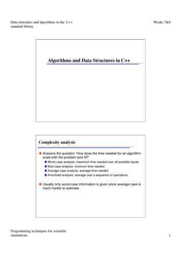
8. Sorting algorithmsGiven an array of unordered entries, we would like to sort the entries so that they are located relative totheir linear ordering.8.1 Introduction to sortingGiven an unsorted list of items that are linearly or weakly ordered, it is often necessary to order the itemsbased on their relative linear ordering. We will assume that the items are stored in an array, and we willdefine a sorting algorithm to be in-place if it uses (1) additional memory (a few local variables). Insome cases, in-place is defined if the additional memory is o(n). There are six sorting design techniqueswe will consider: insertion, selection, exchange, merging, and distribution. We also define a measure ofthe unsortedness of a list, namely, the number of inversions. We look at a very brief overview of a proofthat if a sorting algorithm uses comparison to perform the sort, the binary decision tree must contain n!items, and the minimum average depth of nodes in a binary tree with N nodes is ln(N); consequently, theaverage number of operations is therefore (n ln(n)).8.2 Insertion sortIn order to sort a list, we start with a list of size 1—which is, by definition, sorted—and then given a listof size k, it inserts the next item into the list by placing it into the correct location. Naïvely, the algorithmmay appear to be O(n2); however, a better description is (n d) where d is the number of inversions.The number of comparisons is exactly n d.8.3 Bubble sortWhile having a name catchy name and using a simple idea that appears to be related to insertion sort,bubble sort performs significantly worse than insertion sort. A naïve implementation of the algorithm hasa runtime of (n2), and while various modifications to the algorithm, including alternating betweenbubbling up and sinking down, restricting the search space, etc., the run time can be reduced to (n d)where d is the number of inversions, but unlike insertion sort, the number of comparisons is n 1.5d.8.4 Heap sortIn order to sort a list, we could consider using a priority queue. For example, inserting n items into abinary min-heap using their value to represent their priority requires, at worst, nk 1ln n n ln n time, and taking those same n items out again takes the same amount of time. However, the items willcome out of the heap in order of their values; consequently, the items will come out in linear order. Theonly issue is that this requires (n) additional memory. Instead, converting the array of unsorted itemsinto a binary max-heap, popping the top n times, and placing the popped items into the vacancy left as aresult of the pop allows us to sort the list in place.8.5 Merge sortAnother approach to sorting a list would be to split the list into two, sort each of the halves, and thenmerge the two sorted lists back into one complete sorted list. Merging two lists of size n/2 requires (n)time. If merge sort is applied recursively, we may describe the run time as T(n) 2T(n/2) (n) whenn 1, but this has the additional consequence that the run time is now (n lg(n)) (n ln(n)). We willconsider exactly why the runtime is reduced to this amount when we consider the master theorem in our

topic on divide-and-conquer algorithms. Unfortunately, the merging process requires an additional (n)memory over-and-above the original array.8.6 QuicksortThe most significant issue with merge sort is that it requires (n) additional memory. Instead, anotherapproach would be to find the median element and then rearrange the remaining entries based on whetherthey are less than or greater than the median. We can do this in-place in (n) time, in which case, therun-time would be equal to that of merge sort. Unfortunately, selecting the median is difficult at best.We could randomly choose a pivot, but this would have a tendency of dividing the interval in a ratio of1:3, on average. There would also be a higher likelihood of

9. Hash tables and relation-free storage9.1 Introduction to hash tablesWhen we store linearly ordered data that we intend to both access and modify at arbitrary locations, thisrequires us to use a tree structure that ultimately requires most operations to run in O(ln(n)) time—thelinear ordering prevents us from having run-times that are o(ln(n)). If, however, we don’t care about therelative order (What comes next? What is the largest?), we don’t need the tree structure. Instead, we justneed a simple formula—a hash value—that tells us where to look in an array to find the object. The issueis, it is very difficult to find hash functions that generate unique hash values on a small range from 0 toM – 1, so we must deal with collisions. Our strategy will be to find (1) functions that first map theobject onto a 32-bit number (our hash value), this hash value is mapped to the range 0, , M – 1, andthen deal with collisions.9.2 Hash functionsWe are going to define hash functions as functions that take an object that deterministically takes us to a32-bit value. For example, the address of an object is a 32-bit value which is fine so long as differentobjects are considered to be different under our definition. On the other hand, it is also possible to simplyassign each newly created object a unique hash value in the constructor. For certain objects, twoinstances may be equal under a specific definition (two strings both containing the characters “Hi!”), inwhich case, the hash function must be an arithmetic function of the properties of the object thatdistinguish it in such a way that two equal objects have the same hash value.9.3 Mapping down to 0, , M – 1We are storing objects in an array of size M; consequently, we must map the hash value to that range.Just taking the value modulo M is sub-optimal for a number of reasons. Instead, if we restrict ourselves toarrays that are powers of two (M 2m), it is better to multiply the hash value by a large prime, and thentake the middle m bits.9.4 Chained hash tableThe easiest way to deal with collisions in a hash table is to associate each of the n bin with a linked list orother container. All operations insertion, access, modifications, and erases are performed on theindividual containers associated with the possible hash values. Thus, if the operations on the originalwere, for example, O(n), the corresponding operations on the individual items would be O( ), where isthe load factor.9.6 Open addressingOne issue with using, for example, chained hash tables or scatter tables is that they require (m n)additional memory over-and-above memory required to store the items. This is because an explicitindicator is being used to store a reference to the next bin. Alternatively, an implicit rule could be used toindicate the next location to search.9.7 Linear probingThe easiest rule to follow is to check successive cells in order. In this case, determining membershiprequires us to also follow the same rule until we find the object, find an empty cell, or (in the worst case)iterate through the entire array. Each bin must be marked as either OCCUPIED or UNOCCUPIED. Whenerasing, bins cannot be left empty if there is an object where the empty bin lies on the search path

between the original bin and the bin it is currently stored in. One issue with linear probing is that it leadsto primary clustering: once clusters start growing, they accelerate in their growth leading to longer runtimes.9.9 Double hashingOne solution to the issue of primary clustering seen with linear probing is to give each object a differentjump size. The easiest way to do this is to calculate for each object a second hash value. This jump sizemust be co-prime (relatively prime) with the array size. For array sizes that are powers of two, thisrequires the jump size to be odd. One issue with such a scheme is that it is no longer possible toefficiently determine during an erase what other objects may be appropriately placed into a particular bin.Consequently, each bin must be marked as OCCUPIED, UNOCCUPIED or ERASED.

10. Equivalence relations and disjoint setsAn equivalence relation allows one to break a larger set into equivalence classes. If the larger class isfinite, an equivalence class break

2. Algorithm analysis We describe containers to store items, relationships between items we may also want to record, the concept of abstract data types, data structures and algorithms that will implement these structures and solve problems, and the asymptotic