Transcription
Localization, Mapping, SLAM andThe Kalman Filter according to GeorgeRobotics Institute 16-735http://voronoi.sbp.ri.cmu.edu/ motionHowie Chosethttp://voronoi.sbp.ri.cmu.edu/ chosetRI 16-735, Howie Choset, with slides from George Kantor, G.D. Hager, and D. Fox
The Problem What is the world around me (mapping)– sense from various positions– integrate measurements to produce map– assumes perfect knowledge of position Where am I in the world (localization)–––– senserelate sensor readings to a world modelcompute location relative to modelassumes a perfect world modelTogether, these are SLAM (Simultaneous Localization andMapping)RI 16-735, Howie Choset, with slides from George Kantor, G.D. Hager, and D. Fox
LocalizationTracking: Known initial positionGlobal Localization: Unknown initial positionRe-Localization: Incorrect known position(kidnapped robot or processingPosition estimationControl SchemeExploration SchemeCycle ClosureAutonomyTractabilityScalabilityMapping while tracking locally and globallyRI 16-735, Howie Choset, with slides from George Kantor, G.D. Hager, and D. Fox
Representations for Robot LocalizationKalman filters (late-80s?)Discrete approaches (’95) Topological representation (’95) uncertainty handling (POMDPs) occas. global localization, recovery Grid-based, metric representation (’96) global localization, recoveryParticle filters (’99) sample-based representation global localization, recoveryAI Gaussians approximately linear models position trackingRoboticsMulti-hypothesis (’00) multiple Kalman filters global localization, recoveryRI 16-735, Howie Choset, with slides from George Kantor, G.D. Hager, and D. Fox
Three Major Map ion of discretizedobstacle/free-space pixelsCollection of landmarklocations and correlateduncertaintyCollection of nodes andtheir interconnectionsElfes, Moravec,Thrun, Burgard, Fox,Simmons, Koenig,Konolige, etc.Smith/Self/Cheeseman,Durrant–Whyte, Leonard,Nebot, Christensen, etc.Kuipers/Byun,Chong/Kleeman,Dudek, Choset,Howard, Mataric, etc.RI 16-735, Howie Choset, with slides from George Kantor, G.D. Hager, and D. Fox
Three Major Map ModelsGrid-BasedResolution vs. eature-BasedTopologicalDiscrete localizationArbitrary localizationLocalize to nodesGrid size and resolutionLandmark covariance (N2)Minimal complexityFrontier-basedexplorationNo inherent explorationGraph explorationRI 16-735, Howie Choset, with slides from George Kantor, G.D. Hager, and D. Fox
Atlas Framework Hybrid Solution:– Local features extracted from local grid map.– Local map frames created at complexity limit.– Topology consists of connected local map frames.Authors: Chong, Kleeman; Bosse, Newman, Leonard, Soika, Feiten, TellerRI 16-735, Howie Choset, with slides from George Kantor, G.D. Hager, and D. Fox
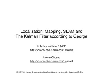
H-SLAMRI 16-735, Howie Choset, with slides from George Kantor, G.D. Hager, and D. Fox
What does a Kalman Filter do, anyway?Given the linear dynamical system:x ( k 1) F ( k ) x ( k ) G ( k )u( k ) v ( k )y ( k ) H ( k ) x ( k ) w( k )x ( k ) is the n - dimensional state vector (unknown)u( k ) is the m - dimensional input vector (known)y ( k ) is the p - dimensional output vector (known, measured)F ( k ), G ( k ), H ( k ) are appropriately dimensioned system matrices (known)v ( k ), w( k ) are zero - mean, white Gaussian noise with (known)covariance matrices Q( k ), R ( k )the Kalman Filter is a recursion that provides the“best” estimate of the state vector x.RI 16-735, Howie Choset, with slides from George Kantor, G.D. Hager, and D. Fox
What’s so great about that?x ( k 1) F ( k ) x ( k ) G ( k )u( k ) v ( k )y ( k ) H ( k ) x ( k ) w( k ) noise smoothing (improve noisy measurements)state estimation (for state feedback)recursive (computes next estimate using only most recent measurement)RI 16-735, Howie Choset, with slides from George Kantor, G.D. Hager, and D. Fox
How does it work?x ( k 1) F ( k ) x ( k ) G ( k )u( k ) v ( k )y ( k ) H ( k ) x ( k ) w( k )1. prediction based on last estimate:xˆ ( k 1 k ) F (k ) xˆ (k k ) G (k )u (k )yˆ (k ) H (k ) xˆ (k 1 k )2. calculate correction based on prediction and current measurement:Δx f ( y (k 1), xˆ (k 1 k ) )3. update prediction:xˆ ( k 1 k 1) xˆ (k 1 k ) ΔxRI 16-735, Howie Choset, with slides from George Kantor, G.D. Hager, and D. Fox
Finding the correction (no noise!)y HxGiven prediction xˆ (k 1 k ) and output y, find Δx so that xˆ xˆ (k 1 k ) Δxis the " best" estimate of x.Want the best estimate to be consistentwith sensor readingsx̂ (k 1 k) Ω {x Hx y}“best” estimate comes from shortest ΔxRI 16-735, Howie Choset, with slides from George Kantor, G.D. Hager, and D. Fox
Finding the correction (no noise!)y HxGiven prediction xˆ (k 1 1) and output y, find Δx so that xˆ xˆ (k 1 1) Δxis the " best" estimate of x.“best” estimate comes from shortest Δxshortest Δx is perpendicular to Ωxˆ (k 1 k ) ΔxΩ {x Hx y}RI 16-735, Howie Choset, with slides from George Kantor, G.D. Hager, and D. Fox
Some linear algebraa is parallel to Ω if Ha 0Null ( H ) {a 0 Ha 0}Ω {x Hx y}a is parallel to Ω if it lies in thenull space of Hfor all v Null ( H ), v b if b column( H T )Weighted sum of columns meansb Hγ , the weighted sum of columnsRI 16-735, Howie Choset, with slides from George Kantor, G.D. Hager, and D. Fox
Finding the correction (no noise!)y HxGiven prediction xˆ (k 1 k ) and output y, find Δx so that xˆ xˆ (k 1 k ) Δxis the " best" estimate of x.“best” estimate comes from shortest Δxshortest Δx is perpendicular to Ωxˆ (k 1 k )T Δx null(H ) Δx column(H ) ΔxΩ {x Hx y} Δx H T γRI 16-735, Howie Choset, with slides from George Kantor, G.D. Hager, and D. Fox
Finding the correction (no noise!)y HxGiven prediction xˆ (k 1 k ) and output y, find Δx so that xˆ xˆ (k 1 k ) Δxis the " best" estimate of x.“best” estimate comes from shortest Δxshortest Δx is perpendicular to Ωxˆ (k 1 k )T Δx null(H ) Δx column(H ) ΔxΩ {x Hx y} Δx H T γReal output – estimated outputν y H ( xˆ (k 1 k )) H ( x xˆ (k 1 k ))innovationRI 16-735, Howie Choset, with slides from George Kantor, G.D. Hager, and D. Fox
Finding the correction (no noise!)y HxGiven prediction xˆ (k 1 k ) and output y, find Δx so that xˆ xˆ (k 1 k ) Δxis the " best" estimate of x.“best” estimate comes from shortest Δxshortest Δx is perpendicular to Ωxˆ (k 1 k )T Δx null(H ) Δx column(H ) ΔxΩ {x Hx y} Δx H T γassume γ is a linear function of ν Δx H T K νGuess, hope, lets face it, it has to be somefunction of the innovationfor some m m matrix KRI 16-735, Howie Choset, with slides from George Kantor, G.D. Hager, and D. Fox
Finding the correction (no noise!)y HxGiven prediction xˆ and output y, find Δx so that xˆ xˆ (k 1 k ) Δxis the " best" estimate of x.we requireH ( xˆ (k 1 k ) Δx) yxˆ (k 1 k ) ΔxΩ {x Hx y}RI 16-735, Howie Choset, with slides from George Kantor, G.D. Hager, and D. Fox
Finding the correction (no noise!)y HxGiven prediction xˆ and output y, find Δx so that xˆ xˆ (k 1 k ) Δxis the " best" estimate of x.we requireH ( xˆ (k 1 k ) Δx) yxˆ (k 1 k ) HΔx y Hxˆ (k 1 k ) H ( x xˆ (k 1 k )) ν ΔxΩ {x Hx y}RI 16-735, Howie Choset, with slides from George Kantor, G.D. Hager, and D. Fox
Finding the correction (no noise!)y HxGiven prediction xˆ and output y, find Δx so that xˆ xˆ (k 1 k ) Δxis the " best" estimate of x.we requireH ( xˆ (k 1 k ) Δx) yxˆ (k 1 k ) HΔx y Hxˆ (k 1 k ) H ( x xˆ (k 1 k )) ν ΔxΩ {x Hx y}substituting Δx H T Kν yieldsHH T Kν νΔx must be perpendicular to Ω b/c anything in therange space of HT is perp to ΩRI 16-735, Howie Choset, with slides from George Kantor, G.D. Hager, and D. Fox
Finding the correction (no noise!)y HxGiven prediction xˆ and output y, find Δx so that xˆ xˆ (k 1 k ) Δxis the " best" estimate of x.we requireH ( xˆ (k 1 k ) Δx) yxˆ (k 1 k ) HΔx y Hxˆ (k 1 k ) H ( x xˆ (k 1 k )) ν ΔxΩ {x Hx y}substituting Δx H T Kν yieldsHH T Kν ν( K HH T) 1The fact that the linear solution solves the equation makes assuming K is linear a kosher guessRI 16-735, Howie Choset, with slides from George Kantor, G.D. Hager, and D. Fox
Finding the correction (no noise!)y HxGiven prediction xˆ and output y, find Δx so that xˆ xˆ (k 1 k ) Δxis the " best" estimate of x.we requireH ( xˆ (k 1 k ) Δx) yxˆ (k 1 k ) HΔx y Hxˆ (k 1 k ) H ( x xˆ (k 1 k )) ν ΔxΩ {x Hx y}substituting Δx H T Kν yieldsHH T Kν ν( K HH TΔx HT) 1(HH )T 1νRI 16-735, Howie Choset, with slides from George Kantor, G.D. Hager, and D. Fox
A Geometric InterpretationΩ {x Hx y}xˆ (k 1 k ) ΔxRI 16-735, Howie Choset, with slides from George Kantor, G.D. Hager, and D. Fox
A Simple State ObserverSystem:x(k 1) Fx(k ) Gu (k )y (k ) Hx(k )1. prediction:xˆ (k 1 k ) Fxˆ (k k ) Gu (k )Observer:2. compute correction:Δx HT(HH )T 1( y (k 1) Hxˆ (k 1 k ))3. update:xˆ ( k 1 k 1) xˆ (k 1 k ) ΔxRI 16-735, Howie Choset, with slides from George Kantor, G.D. Hager, and D. Fox
Caveat #1Note: The observer presented here is not a very goodobserver. Specifically, it is not guaranteed to converge forall systems. Still the intuition behind this observer is thesame as the intuition behind the Kalman filter, and theproblems will be fixed in the following slides.It really corrects only to the current sensor information,so if you are on the hyperplane but not at right place, youhave no correction . I am waiving my hands here, look in bookRI 16-735, Howie Choset, with slides from George Kantor, G.D. Hager, and D. Fox
Estimating a distribution for xOur estimate of x is not exact!We can do better by estimating a joint Gaussian distribution p(x).p( x) ((1(2π ) n / 2 Pwhere P E ( x xˆ )( x xˆ ) T)1/ 2 1( x xˆ )T P 1 ( x xˆ )e2)is the covariance matrixRI 16-735, Howie Choset, with slides from George Kantor, G.D. Hager, and D. Fox
Finding the correction (geometric intuition)Given prediction xˆ (k 1 k ), covariance P, and output y , find Δx so thatxˆ xˆ (k 1 k ) Δx is the " best" (i.e. most probable) estimate of x.Ω {x Hx y}xˆ (k 1 k )Δxp( x) (1(2π ) n / 2 P1/ 2 1( x xˆ )T P 1 ( x xˆ )e2)The most probable Δx is the one that :1. satisfies xˆ ( k 1 k 1) xˆ (k 1 k ) Δx2. minimizes ΔxT P 1ΔxRI 16-735, Howie Choset, with slides from George Kantor, G.D. Hager, and D. Fox
A new kind of distanceSuppose we define a new inner product on R n to be :x1 , x2 x1T P 1 x 2(this replaces the old inner product x1T x2 )Then we can define a new norm x2 x , x x T P 1 xThe xˆ in Ω that minimizes Δx is the orthogonal projection of xˆ (k 1 k )onto Ω, so Δx is orthogonal to Ω. ω , Δx 0 for ω in TΩ null ( H )ω , Δx ω T P 1Δx 0 iff Δx column ( PH T )RI 16-735, Howie Choset, with slides from George Kantor, G.D. Hager, and D. Fox
Finding the correction (for real this time!)Assuming that Δx is linear in ν y Hxˆ ( k 1 k )Δx PH T KνThe condition y H ( xˆ (k 1 k ) Δx ) HΔx y Hxˆ (k 1 k ) νSubstituti on yields :HΔx ν HPH T Kν( K HPH Δx PHTT) 1(HPH )T 1νRI 16-735, Howie Choset, with slides from George Kantor, G.D. Hager, and D. Fox
A Better State Observerx(k 1) Fx(k ) Gu (k ) v(k )y (k ) Hx(k )Sample of Guassian Dist. w/COV QWe can create a better state observer following the same 3. steps, but now wemust also estimate the covariance matrix P.We start with x(k k) and P(k k)Where did noise go?Expected value Step 1: Predictionxˆ (k 1 k ) Fxˆ (k k ) Gu (k )What about P? From the definition:(P ( k k ) E ( x (k ) xˆ (k k ))( x(k ) xˆ (k k ))Tand)(P ( k 1 k ) E ( x(k 1) xˆ (k 1 k ))( x(k 1) xˆ (k 1 k ))TRI 16-735, Howie Choset, with slides from George Kantor, G.D. Hager, and D. Fox)
Continuing Step 1To make life a little easier, lets shift notation slightly:(Pk 1 E ( xk 1 xˆ k 1 )( xk 1 xˆ k 1 )T)( E ((F (x xˆ ) v )(F (x xˆ ) v ) ) E (F (x xˆ )(x xˆ ) F 2 F (x xˆ )v FE ((x xˆ )(x xˆ ) )F E (v v ) E (Fx k Gu k vk ( Fxˆ k Gu k ) )(Fx k Gu k vk ( Fxˆ k Gu k ) )TTkkkkTkkkkkkTkkTkkkTkTk v k v Tk)Tkk FPk F T QP (k 1 k ) FP (k k ) F T QRI 16-735, Howie Choset, with slides from George Kantor, G.D. Hager, and D. Fox)
Step 2: Computing the correctionFrom step 1 we get xˆ ( k 1 k ) and P (k 1 k ).Now we use these to compute Δx :(Δx P ( k 1 k ) H HP ( k 1 k ) HT) 1( y (k 1) Hxˆ (k 1 k ) )For ease of notation, define W so thatΔx WνRI 16-735, Howie Choset, with slides from George Kantor, G.D. Hager, and D. Fox
Step 3: Updatexˆ ( k 1 k 1) xˆ ( k 1 k ) Wν( E (( xPk 1 E ( x k 1 xˆ k 1 )( x k 1 xˆ k 1 )T) Tˆˆ x Wν)(x x Wν)k 1k 1k 1k 1)(just take my word for it )P (k 1 k 1) P (k 1 k ) WHP (k 1 k ) H T W TRI 16-735, Howie Choset, with slides from George Kantor, G.D. Hager, and D. Fox
Just take my word for it ( E (( x E (( x Pk 1 E ( x k 1 xˆ k 1 )( x k 1 xˆ k 1 )Tk 1))) Wν ) xˆ k 1 Wν )( xk 1 xˆ k 1 Wν )T)(ˆ k 1 ) Wν ( xk 1 xˆ k 1k 1 xT( E ( xk 1 xˆ k 1 )( xk 1 xˆ k 1 )T 2Wν ( xk 1 xˆ k 1 )T Wν (Wν )T)( Pk 1 E 2WH ( xk 1 xˆ k 1 )( xk 1 xˆ k 1 )T WH ( xk 1 xˆ k 1 )( xk 1 xˆ k 1 )T H T W T Pk 1 2WHPk 1 WHPk 1 H T W T((HP Pk 1 2 Pk 1 H T HPk 1 H T Pk 1 2 Pk 1 H T) HP) (HP 1 T 1Hk 1 k 1 WHPk 1 H T W T Tk 1 H)(HP) T 1HHPk 1k 1 WHPk 1 H T W T Pk 1 2WHPk 1 H T W T WHPk 1 H T W TRI 16-735, Howie Choset, with slides from George Kantor, G.D. Hager, and D. Fox)
Better State Observer SummarySystem:1. Predictx(k 1) Fx(k ) Gu (k ) v(k )y (k ) Hx(k )xˆ (k 1 k ) Fxˆ (k k ) Gu (k )ObserverP (k 1 k ) FP (k k ) F T Q2. Correction3. Update(W P (k 1 k ) H HP (k 1 k ) H TΔx W ( y ( k 1) Hxˆ (k 1 k ) )) 1xˆ ( k 1 k 1) xˆ ( k 1 k ) WνP (k 1 k 1) P (k 1 k ) WHP (k 1 k ) H T W TRI 16-735, Howie Choset, with slides from George Kantor, G.D. Hager, and D. Fox
Note: there is a problem with the previous slide, namely the covariance matrix ofthe estimate P will be singular. This makes sense because with perfect sensormeasurements the uncertainty in some directions will be zero. There is nouncertainty in the directions perpendicular to ΩP lives in the state space and directions associated with sensor noise are zero. Inthe step when you do the update, if you have a zero noise measurement, you endup squeezing P down.In most cases, when you do the next prediction step, the process covariance matrixQ gets added to the P(k k), the result will be nonsingular, and everything is ok again.There’s actually not anything wrong with this, except that you can’t really call theresult a “covariance” matrix because “sometimes” it is not a covariance matrixPlus, lets not be ridiculous, all sensors have noise.RI 16-735, Howie Choset, with slides from George Kantor, G.D. Hager, and D. Fox
Finding the correction (with output noise)y Hx wΩ {x Hx y}The previous results require that you knowwhich hyperplane to aim for. Because thereis now sensor noise, we don’t know where toaim, so we can’t directly use our method.If. we can determine which hyperplane aimfor, then the previous result would apply.xˆ (k 1 k )We find the hyperplane in question as follows:1.2.3.project estimate into output spacefind most likely point in output space based onmeasurement and projected predictionthe desired hyperplane is the preimage of this pointRI 16-735, Howie Choset, with slides from George Kantor, G.D. Hager, and D. Fox
Projecting the prediction(putting current state estimates into sensor space)xˆ (k 1 k ) yˆ Hxˆ (k 1 k )P (k 1 k ) Rˆ HP(k 1 k ) H TP(k 1 k )xˆ (k 1 k ) state space (n-dimensional)R̂ŷ output space (p-dimensional)RI 16-735, Howie Choset, with slides from George Kantor, G.D. Hager, and D. Fox
Finding most likely outputence independent, so multiply them because we want them both to be true at the same timeThe objective is to find the most likely output that resultsfrom the independent Gaussian distributions( y, R) measurement and associate covariance( yˆ , Rˆ ) projected prediction (what you think your measurementsshould be and how confident you are)Fact (Kalman Gains): The product of two Gaussian distributions given bymean/covariance pairs (x1,C1) and (x2,C2) is proportional to a third Gaussianwith meanx3 x1 K ( x2 x1 )and covariancewhereC3 C1 KC1K C1 (C1 C2 ) 1Strange, but true,this is symmetricRI 16-735, Howie Choset, with slides from George Kantor, G.D. Hager, and D. Fox
Most likely output (cont.)Using the Kalman gains, the most likely output is(y yˆ Rˆ Rˆ R *(() 1 ( yˆ y ) Hxˆ (k 1 k ) HPH HPH RTT) 1)(Hxˆ(k 1 k ) y)RI 16-735, Howie Choset, with slides from George Kantor, G.D. Hager, and D. Fox
Finding the CorrectionNow we can compute the correction as we did in the noiseless case, this timeusing y* instead of y. In other words, y* tells us which hyperplane to aim for.{Ω x Hx y *}The result is:x̂ Δx(Δx PH HPHTT) (y 1* Hxˆ ( k 1 k )ot going all the way to y, but splitting the difference between how confident you are with yourSensor and process noiseRI 16-735, Howie Choset, with slides from George Kantor, G.D. Hager, and D. Fox)
Finding the Correction (cont.)() (y Hxˆ (k 1 k ))) (Hxˆ HPH (HPH R ) ( y Hxˆ (k 1 k )) Hxˆ (k 1 k ))Δx PH HPHT( PH T HPH T( 1T* 1 PH HPH RTTTT 1) ( y Hxˆ (k 1 k )) 1For convenience, we define(W PH HPH RTT) 1So thatΔx W ( y Hxˆ ( k 1 k ) )RI 16-735, Howie Choset, with slides from George Kantor, G.D. Hager, and D. Fox
Correcting the Covariance EstimateThe covariance error estimate correction is computed fromthe definition of the covariance matrix, in much the sameway that we computed the correction for the “betterobserver”. The answer turns out to be:()P (k 1 k 1) P (k 1 k ) W HP (k 1 k ) H WRI 16-735, Howie Choset, with slides from George Kantor, G.D. Hager, and D. FoxTT
LTI Kalman Filter SummarySystem:Kalman Filter1. Predictx(k 1) Fx(k ) Gu (k ) v(k )y (k ) Hx(k ) w(k )xˆ (k 1 k ) Fxˆ (k k ) Gu (k )P (k 1 k ) FP (k k ) F T QS HP ( k 1 k ) H T R2. Correction3. UpdateW P ( k 1 k ) H T S 1Δx W ( y ( k 1) Hxˆ (k 1 k ) )xˆ ( k 1 k 1) xˆ ( k 1 k ) WνP (k 1 k 1) P (k 1 k ) WSW TRI 16-735, Howie Choset, with slides from George Kantor, G.D. Hager, and D. Fox
Kalman FiltersRI 16-735, Howie Choset, with slides from George Kantor, G.D. Hager, and D. Fox
Kalman Filter for Dead Reckoning Robot moves along a straight line with state x [xr, vr]T u is the force applied to the robot Newton tells usorProcess noisefrom a zeromeanGaussian V Robot has velocity sensorSensor noise from azero mean Gaussian WRI 16-735, Howie Choset, with slides from George Kantor, G.D. Hager, and D. Fox
Set upAssumeAt some time kPUT ELLIPSE FIGURE HERERI 16-735, Howie Choset, with slides from George Kantor, G.D. Hager, and D. Fox
ObservabilityRecall from last timeActually, previous example is not observable but still nice to use Kalman filterRI 16-735, Howie Choset, with slides from George Kantor, G.D. Hager, and D. Fox
Extended Kalman Filter Life is not linear PredictRI 16-735, Howie Choset, with slides from George Kantor, G.D. Hager, and D. Fox
Extended Kalman Filter UpdateRI 16-735, Howie Choset, with slides from George Kantor, G.D. Hager, and D. Fox
EKF for Range-Bearing Localization Stateposition and orientation Inputforward and rotational velocity Process Model nl landmarkscan only see p(k) of them at kAssociation mapRI 16-735, Howie Choset, with slides from George Kantor, G.D. Hager, and D. Fox
Be wise, and linearize.RI 16-735, Howie Choset, with slides from George Kantor, G.D. Hager, and D. Fox
Data Association BIG PROBLEMIth measurement corresponds to the jth landmarkinnovationwherePick the smallestRI 16-735, Howie Choset, with slides from George Kantor, G.D. Hager, and D. Fox
Kalman Filter for SLAM (simple)stateInputs are commands to x and y velocities, a bit naiveProcess modelRI 16-735, Howie Choset, with slides from George Kantor, G.D. Hager, and D. Fox
Kalman Filter for SLAMRI 16-735, Howie Choset, with slides from George Kantor, G.D. Hager, and D. Fox
Range BearingInputs are forward and rotational velocitiesRI 16-735, Howie Choset, with slides from George Kantor, G.D. Hager, and D. Fox
Greg’s Notes: Some Examples Point moving on the line according to f m a– state is position and velocity– input is force– sensing should be position Point in the plane under Newtonian laws Nonholonomic kinematic system (no dynamics)– state is workspace configuration– input is velocity command– sensing could be direction and/or distance to beacons Note that all of dynamical systems are “open-loop” integrationRole of sensing is to “close the loop” and pin down stateRI 16-735, Howie Choset, with slides from George Kantor, G.D. Hager, and D. Fox
Kalman FiltersBel ( xt ) N ( μ t , σ t2 ) μt 1 μt But Bel(xt 1 ) 22 22σ Aσ σtact t 1 μt 1 μt 1 K t 1 ( μ zt 1 μt 1 )Bel(xt 1 ) σ t2 1 (1 K t 1 )σ t2 1 μt 2 μt 1 But 1 Bel(xt 2 ) 22 22σ Aσ σt 1act t 2RI 16-735, Howie Choset, with slides from George Kantor, G.D. Hager, and D. Fox
Kalman Filter Algorithm1.Algorithm Kalman filter( μ,Σ , d ):2.3.4.5.If d is a perceptual data item y then6.7.8.Else if d is an action data item u thenμ Aμ Bu9.Return μ,Σ (K ΣC CΣC Σ obsμ μ K ( z Cμ )TT) 1Σ ( I KC )ΣΣ AΣAT Σ actRI 16-735, Howie Choset, with slides from George Kantor, G.D. Hager, and D. Fox
Limitations Very strong assumptions:– Linear state dynamics– Observations linear in state What can we do if system is not linear?– Non-linear state dynamics– Non-linear observationsX t 1 AX t But Σ actZ t CX t Σ obsX t 1 f ( X t , ut , Σ act )Z t c( X t , Σ obs ) Linearize it! Determine Jacobians of dynamics f and observationfunction c w.r.t the current state x and the noise.Aij c f i ci f i( xt , ut ,0) Cij i ( xt ,0) Wij ( xt , ut ,0) Vij ( xt ,0) x j x j Σ act j Σ obs jRI 16-735, Howie Choset, with slides from George Kantor, G.D. Hager, and D. Fox
Extended Kalman Filter Algorithm1.Algorithm Extended Kalman filter( μ,Σ , d):2.3.4.5.If d is a perceptual data item z then6.7.8.Else if d is an action data item u thenμ f ( μ , u , 0)μ Aμ Bu9.Return μ,Σ (K ΣC CΣC VΣ obsVμ μ K (z c( μ ,0) )Σ ( I KC )ΣTTΣ AΣAT WΣ actW T)T 1(K ΣC CΣC Σ obsμ μ K ( z Cμ )TTΣ ( I KC )ΣΣ AΣAT Σ actRI 16-735, Howie Choset, with slides from George Kantor, G.D. Hager, and D. Fox) 1
Kalman Filter-based Systems (2) [Arras et al. 98]: Laser range-finder and vision High precision ( 1cm accuracy)Courtesy of RIK. 16-735,Arras Howie Choset, with slides from George Kantor, G.D. Hager, and D. Fox
Unscented Kalman Filter Instead of linearizing, pass several points from the Gaussian through the nonlinear transformation and re-compute a new Gaussian.Better performance (theory and practice).μμ ' f ( μ , u ,0)Σ AΣAT WΣ actW Tμffμ’μ’RI 16-735, Howie Choset, with slides from George Kantor, G.D. Hager, and D. Fox
Kalman Filters and SLAM Localization: state is the location of the robot Mapping: state is the location of beacons SLAM: state combines both Consider a simple fully-observable holonomic robot– x(k 1) x(k) u(k) dt v– yi(k) pi - x(k) w If the state is (x(k),p1, p2 .) then we can write a linear observationsystem– note that if we don’t have some fixed beacons, our system is unobservable(we can’t fully determine all unknown quantities)RI 16-735, Howie Choset, with slides from George Kantor, G.D. Hager, and D. Fox
The fact that the linear solution solves the equation makes assuming K is linear a kosher guess RI 16-735, Howie Choset, with slides from George Kantor,