Transcription
A Practical Guide toWavelet AnalysisChristopher Torrence and Gilbert P. CompoProgram in Atmospheric and Oceanic Sciences, University of Colorado, Boulder, ColoradoABSTRACTA practical step-by-step guide to wavelet analysis is given, with examples taken from time series of the El Niño–Southern Oscillation (ENSO). The guide includes a comparison to the windowed Fourier transform, the choice of anappropriate wavelet basis function, edge effects due to finite-length time series, and the relationship between waveletscale and Fourier frequency. New statistical significance tests for wavelet power spectra are developed by deriving theoretical wavelet spectra for white and red noise processes and using these to establish significance levels and confidenceintervals. It is shown that smoothing in time or scale can be used to increase the confidence of the wavelet spectrum.Empirical formulas are given for the effect of smoothing on significance levels and confidence intervals. Extensions towavelet analysis such as filtering, the power Hovmöller, cross-wavelet spectra, and coherence are described.The statistical significance tests are used to give a quantitative measure of changes in ENSO variance on interdecadaltimescales. Using new datasets that extend back to 1871, the Niño3 sea surface temperature and the Southern Oscillation index show significantly higher power during 1880–1920 and 1960–90, and lower power during 1920–60, as wellas a possible 15-yr modulation of variance. The power Hovmöller of sea level pressure shows significant variations in2–8-yr wavelet power in both longitude and time.1. IntroductionWavelet analysis is becoming a common tool foranalyzing localized variations of power within a timeseries. By decomposing a time series into time–frequency space, one is able to determine both the dominant modes of variability and how those modes varyin time. The wavelet transform has been used for numerous studies in geophysics, including tropical convection (Weng and Lau 1994), the El Niño–SouthernOscillation (ENSO; Gu and Philander 1995; Wang andWang 1996), atmospheric cold fronts (Gamage andBlumen 1993), central England temperature (Baliunaset al. 1997), the dispersion of ocean waves (Meyers etal. 1993), wave growth and breaking (Liu 1994), andcoherent structures in turbulent flows (Farge 1992). ACorresponding author address: Dr. Christopher Torrence, Advanced Study Program, National Center for Atmospheric Research, P.O. Box 3000, Boulder, CO 80307-3000.E-mail: torrence@ucar.eduIn final form 20 October 1997. 1998 American Meteorological SocietyBulletin of the American Meteorological Societycomplete description of geophysical applications canbe found in Foufoula-Georgiou and Kumar (1995),while a theoretical treatment of wavelet analysis isgiven in Daubechies (1992).Unfortunately, many studies using wavelet analysis have suffered from an apparent lack of quantitative results. The wavelet transform has been regardedby many as an interesting diversion that produces colorful pictures, yet purely qualitative results. This misconception is in some sense the fault of wavelet analysis itself, as it involves a transform from a one-dimensional time series (or frequency spectrum) to a diffusetwo-dimensional time–frequency image. This diffuseness has been exacerbated by the use of arbitrary normalizations and the lack of statistical significance tests.In Lau and Weng (1995), an excellent introductionto wavelet analysis is provided. Their paper, however,did not provide all of the essential details necessaryfor wavelet analysis and avoided the issue of statistical significance.The purpose of this paper is to provide an easy-touse wavelet analysis toolkit, including statistical significance testing. The consistent use of examples of61
a. NINO3 88.01616.03232.0641880190019201940Time (year)19601980Scale (years)Period (years)0.5164.02000c. 201940Time (year)19601980Scale (years)0.125116.0002000FIG. 1. (a) The Niño3 SST time series used for the wavelet analysis. (b) Thelocal wavelet power spectrum of (a) using the Morlet wavelet, normalized by 1/σ2 (σ2 0.54 C2). The left axis is the Fourier period (in yr) corresponding to thewavelet scale on the right axis. The bottom axis is time (yr). The shaded contoursare at normalized variances of 1, 2, 5, and 10. The thick contour encloses regionsof greater than 95% confidence for a red-noise process with a lag-1 coefficient of0.72. Cross-hatched regions on either end indicate the “cone of influence,” whereedge effects become important. (c) Same as (b) but using the real-valued Mexicanhat wavelet (derivative of a Gaussian; DOG m 2). The shaded contour is atnormalized variance of 2.0.2. DataSeveral time series will be used for examples ofwavelet analysis. These include the Niño3 sea surfacetemperature (SST) used as a measure of the amplitudeof the El Niño–Southern Oscillation (ENSO). TheNiño3 SST index is defined as the seasonal SST averaged over the central Pacific (5 S–5 N, 90 –150 W). Data for 1871–1996 are from an area average of the U.K. Meteorological Office GISST2.3(Rayner et al. 1996), while data for January–June 1997are from the Climate Prediction Center (CPC) optimally interpolated Niño3 SST index (courtesy of D.Garrett at CPC, NOAA). The seasonal means for the621900b. MorletPeriod (years)ENSO provides a substantive addition tothe ENSO literature. In particular, thestatistical significance testing allowsgreater confidence in the previous wavelet-based ENSO results of Wang andWang (1996). The use of new datasetswith longer time series permits a morerobust classification of interdecadalchanges in ENSO variance.The first section describes the datasetsused for the examples. Section 3 describes the method of wavelet analysisusing discrete notation. This includes adiscussion of the inherent limitations ofthe windowed Fourier transform (WFT),the definition of the wavelet transform,the choice of a wavelet basis function,edge effects due to finite-length time series, the relationship between waveletscale and Fourier period, and time seriesreconstruction. Section 4 presents thetheoretical wavelet spectra for bothwhite-noise and red-noise processes.These theoretical spectra are compared toMonte Carlo results and are used to establish significance levels and confidence intervals for the wavelet powerspectrum. Section 5 describes time orscale averaging to increase significancelevels and confidence intervals. Section6 describes other wavelet applicationssuch as filtering, the power Hovmöller,cross-wavelet spectra, and wavelet coherence. The summary contains a stepby-step guide to wavelet analysis.entire record have been removed to define an anomalytime series. The Niño3 SST is shown in the top plotof Fig. 1a.Gridded sea level pressure (SLP) data is from theUKMO/CSIRO historical GMSLP2.1f (courtesy of D.Parker and T. Basnett, Hadley Centre for Climate Prediction and Research, UKMO). The data is on a 5 global grid, with monthly resolution from January1871 to December 1994. Anomaly time series havebeen constructed by removing the first three harmonics of the annual cycle (periods of 365.25, 182.625, and121.75 days) using a least-squares fit.The Southern Oscillation index is derived from theGMSLP2.1f and is defined as the seasonally averagedpressure difference between the eastern Pacific (20 S,150 W) and the western Pacific (10 S, 130 E).Vol. 79, No. 1, January 1998
3. Wavelet analysisThis section describes the method of wavelet analysis, includes a discussion of different wavelet functions, and gives details for the analysis of the waveletpower spectrum. Results in this section are adapted todiscrete notation from the continuous formulas givenin Daubechies (1990). Practical details in applyingwavelet analysis are taken from Farge (1992), Wengand Lau (1994), and Meyers et al. (1993). Each section is illustrated with examples using the Niño3 SST.ψ (t / s) ψ(s ω)a. Morlet0.3640.0-0.3-42-2024b. Paul (m 4)0.30-2-10126a. Windowed Fourier transformThe WFT represents one analysis tool for extracting local-frequency information from a signal. TheFourier transform is performed on a sliding segmentof length T from a time series of time step δt and totallength Nδ t, thus returning frequencies from T 1 to(2δt) 1 at each time step. The segments can be windowed with an arbitrary function such as a boxcar (nosmoothing) or a Gaussian window (Kaiser 1994).As discussed by Kaiser (1994), the WFT representsan inaccurate and inefficient method of time–frequency localization, as it imposes a scale or “responseinterval” T into the analysis. The inaccuracy arisesfrom the aliasing of high- and low-frequency components that do not fall within the frequency range of thewindow. The inefficiency comes from the T/(2δt) frequencies, which must be analyzed at each time step,regardless of the window size or the dominant frequencies present. In addition, several window lengths mustusually be analyzed to determine the most appropriate choice. For analyses where a predetermined scaling may not be appropriate because of a wide rangeof dominant frequencies, a method of time–frequencylocalization that is scale independent, such as wavelet analysis, should be employed.40.0-0.3-42-2024c. DOG (m 2)0.30-2-1012-1012640.0-0.3-42-2024d. DOG (m 6)0.30-26ψ 0 (η) π 1 4 e iω 0η e η40.0-0.3-4b. Wavelet transformThe wavelet transform can be used to analyze timeseries that contain nonstationary power at many different frequencies (Daubechies 1990). Assume thatone has a time series, xn, with equal time spacing δtand n 0 N 1. Also assume that one has a wavelet function, ψ0(η), that depends on a nondimensional“time” parameter η. To be “admissible” as a wavelet,this function must have zero mean and be localized inboth time and frequency space (Farge 1992). An example is the Morlet wavelet, consisting of a planewave modulated by a Gaussian:22,(1)2-20t/s240-2-1012s ω / (2π)FIG. 2. Four different wavelet bases, from Table 1. The plotson the left give the real part (solid) and imaginary part (dashed)for the wavelets in the time domain. The plots on the right givethe corresponding wavelets in the frequency domain. For plottingpurposes, the scale was chosen to be s 10δt. (a) Morlet, (b) Paul(m 4), (c) Mexican hat (DOG m 2), and (d) DOG (m 6).Bulletin of the American Meteorological Societywhere ω0 is the nondimensional frequency, here takento be 6 to satisfy the admissibility condition (Farge1992). This wavelet is shown in Fig. 2a.The term “wavelet function” is used generically torefer to either orthogonal or nonorthogonal wavelets.The term “wavelet basis” refers only to an orthogonal set of functions. The use of an orthogonal basisimplies the use of the discrete wavelet transform,while a nonorthogonal wavelet function can be used63
with either the discrete or the continuous wavelettransform (Farge 1992). In this paper, only the continuous transform is used, although all of the resultsfor significance testing, smoothing in time and scale,and cross wavelets are applicable to the discrete wavelet transform.The continuous wavelet transform of a discrete sequence xn is defined as the convolution of xn with ascaled and translated version of ψ0(η):Wn ( s) (n ′ n)δ t x n ′ψ ,s n ′ 0N 1 (2)where the (*) indicates the complex conjugate. Byvarying the wavelet scale s and translating along thelocalized time index n, one can construct a pictureshowing both the amplitude of any features versus thescale and how this amplitude varies with time. Thesubscript 0 on ψ has been dropped to indicate that thisψ has also been normalized (see next section). Although it is possible to calculate the wavelet transformusing (2), it is considerably faster to do the calculations in Fourier space.To approximate the continuous wavelet transform,the convolution (2) should be done N times for eachscale, where N is the number of points in the time series (Kaiser 1994). (The choice of doing all N convolutions is arbitrary, and one could choose a smallernumber, say by skipping every other point in n.) Bychoosing N points, the convolution theorem allows usdo all N convolutions simultaneously in Fourier spaceusing a discrete Fourier transform (DFT). The DFTof xn is1x̂ k NN 1 x e 2 πikn Nn,(3)n 0where k 0 N 1 is the frequency index. In thecontinuous limit, the Fourier transform of a functionψ(t/s) is given by ψ (sω). By the convolution theorem,the wavelet transform is the inverse Fourier transformof the product: 2π k : k N Nδ t2ω k 2π kN. : k Nδ t2(5)Using (4) and a standard Fourier transform routine, onecan calculate the continuous wavelet transform (for agiven s) at all n simultaneously and efficiently.c. NormalizationTo ensure that the wavelet transforms (4) at eachscale s are directly comparable to each other and to thetransforms of other time series, the wavelet functionat each scale s is normalized to have unit energy:12 2π s ψˆ (sω k ) ψˆ 0 ( sω k ) . δt (6)Examples of different wavelet functions are given inTable 1 and illustrated in Fig. 2. Each of the unscaledψ 0 are defined in Table 1 to have ψˆ 0 (ω ′ ) dω ′ 1 ;2that is, they have been normalized to have unit energy.Using these normalizations, at each scale s one hasN 1 ψ̂ (sω )2k N,(7)k 0where N is the number of points. Thus, the wavelettransform is weighted only by the amplitude of theFourier coefficients x k and not by the wavelet function.If one is using the convolution formula (2), the normalization is (n ′ n)δ t δ t (n ′ n)δ t ψ0 ψ ,ss s 12(8)where ψ0(η) is normalized to have unit energy.Wn ( s) N 1 xˆ ψ̂ (sω )ekkiω k nδ t,k 0where the angular frequency is defined as64(4)d. Wavelet power spectrumBecause the wavelet function ψ (η) is in generalcomplex, the wavelet transform Wn(s) is also complex.The transform can then be divided into the real part,Vol. 79, No. 1, January 1998
TABLE 1. Three wavelet basis functions and their properties. Constant factors for ψ0 and ψ 0 ensure a total energy of unity.Morlet(ω0 frequency)π 1 4 e iω 0η e η2 m i m m!Paul(m order)π ( 2 m )!( 1) m 1DOG(m derivative)e-foldingtime τs ψ0(η)Nameψ 0(sω)22 sω ω 0 )π 1 4 H (ω )e (22m(1 iη) ( m 1)(d m η 2em1 dηΓ m 2 2)4πs22sH (ω )( sω ) e sωmm(2 m 1)! im1Γ m 2 Fourierwavelength λ(sω ) m e ( sω )2s2ω 0 2 ω 204π s2m 12π s22sm 12H(ω) Heaviside step function, H(ω) 1 if ω 0, H(ω) 0 otherwise.DOG derivative of a Gaussian; m 2 is the Marr or Mexican hat wavelet.ℜ{Wn(s)}, and imaginary part, ℑ{Wn(s)}, or amplitude, Wn(s) , and phase, tan 1[ℑ{Wn(s)}/ℜ{Wn(s)}]. Finally, one can define the wavelet power spectrum as Wn(s) 2. For real-valued wavelet functions such as theDOGs (derivatives of a Gaussian) the imaginary partis zero and the phase is undefined.To make it easier to compare different waveletpower spectra, it is desirable to find a common normalization for the wavelet spectrum. Using the normalization in (6), and referring to (4), the expectationvalue for Wn(s) 2 is equal to N times the expectationvalue for x k 2. For a white-noise time series, this expectation value is σ2/N, where σ2 is the variance. Thus,for a white-noise process, the expectation value for thewavelet transform is Wn(s) 2 σ 2 at all n and s.Figure 1b shows the normalized wavelet powerspectrum, Wn(s) 2/σ 2, for the Niño3 SST time series.The normalization by 1/σ 2 gives a measure of thepower relative to white noise. In Fig. 1b, most of thepower is concentrated within the ENSO band of 2–8yr, although there is appreciable power at longer periods. The 2–8-yr band for ENSO agrees with other studBulletin of the American Meteorological Societyies (Trenberth 1976) and is also seen in the Fourierspectrum in Fig. 3. With wavelet analysis, one can seevariations in the frequency of occurrence and amplitude of El Niño (warm) and La Niña (cold) events.During 1875–1920 and 1960–90 there were manywarm and cold events of large amplitude, while during 1920–60 there were few events (Torrence andWebster 1997). From 1875–1910, there was a slightshift from a period near 4 yr to a period closer to 2 yr,while from 1960–90 the shift is from shorter to longerperiods.These results are similar to those of Wang andWang (1996), who used both wavelet and waveformanalysis on ENSO indices derived from the Comprehensive Ocean–Atmosphere Data Set (COADS)dataset. Wang and Wang’s analysis showed reducedwavelet power before 1950, especially 1875–1920. Thereduced power is possibly due to the sparseness and decreased reliability of the pre-1950 COADS data (Follandet al. 1984). With the GISST2.3 data, the wavelet transform of Niño3 SST in Fig. 1b shows that the pre-1920period has equal power to the post-1960 period.65
14Variance (σ2)121086420643216842Period (years)10.5F IG . 3. Fourier power spectrum of Niño3 SST (solid),normalized by N/(2σ 2). The lower dashed line is the mean rednoise spectrum from (16) assuming a lag-1 of α 0.72. The upperdashed line is the 95% confidence spectrum.e. Wavelet functionsOne criticism of wavelet analysis is the arbitrarychoice of the wavelet function, ψ0(η). (It should benoted that the same arbitrary choice is made in usingone of the more traditional transforms such as the Fourier, Bessel, Legendre, etc.) In choosing the waveletfunction, there are several factors which should beconsidered (for more discussion see Farge 1992).1) Orthogonal or nonorthogonal. In orthogonalwavelet analysis, the number of convolutions ateach scale is proportional to the width of the wavelet basis at that scale. This produces a wavelet spectrum that contains discrete “blocks” of waveletpower and is useful for signal processing as it givesthe most compact representation of the signal. Unfortunately for time series analysis, an aperiodicshift in the time series produces a different wavelet spectrum. Conversely, a nonorthogonal analysis (such as used in this study) is highly redundantat large scales, where the wavelet spectrum at adjacent times is highly correlated. The nonorthogonal transform is useful for time series analysis,where smooth, continuous variations in waveletamplitude are expected.2) Complex or real. A complex wavelet function willreturn information about both amplitude and phase66and is better adapted for capturing oscillatory behavior. A real wavelet function returns only asingle component and can be used to isolate peaksor discontinuities.3) Width. For concreteness, the width of a waveletfunction is defined here as the e-folding time of thewavelet amplitude. The resolution of a waveletfunction is determined by the balance between thewidth in real space and the width in Fourier space.A narrow (in time) function will have good timeresolution but poor frequency resolution, while abroad function will have poor time resolution, yetgood frequency resolution.4) Shape. The wavelet function should reflect the typeof features present in the time series. For time series with sharp jumps or steps, one would choosea boxcar-like function such as the Harr, while forsmoothly varying time series one would choose asmooth function such as a damped cosine. If oneis primarily interested in wavelet power spectra,then the choice of wavelet function is not critical,and one function will give the same qualitativeresults as another (see discussion of Fig. 1 below).Four common nonorthogonal wavelet functions aregiven in Table 1. The Morlet and Paul wavelets areboth complex, while the DOGs are real valued. Pictures of these wavelet in both the time and frequencydomain are shown in Fig. 2. Many other types of wavelets exist, such as the Haar and Daubechies, most ofwhich are used for orthogonal wavelet analysis (e.g.,Weng and Lau 1994; Mak 1995; Lindsay et al. 1996).For more examples of wavelet bases and functions, seeKaiser (1994).For comparison, Fig. 1c shows the same analysisas in 1b but using the Mexican hat wavelet (DOG,m 2) rather than the Morlet. The most noticeable difference is the fine scale structure using the Mexicanhat. This is because the Mexican hat is real valued andcaptures both the positive and negative oscillations ofthe time series as separate peaks in wavelet power. TheMorlet wavelet is both complex and contains moreoscillations than the Mexican hat, and hence the wavelet power combines both positive and negative peaksinto a single broad peak. A plot of the real or imaginary part of Wn(s) using the Morlet would produce aplot similar to Fig. 1c. Overall, the same features appear in both plots, approximately at the same locations,and with the same power. Comparing Figs. 2a and 2c,the Mexican hat is narrower in time-space, yet broaderin spectral-space than the Morlet. Thus, in Fig. 1c, theVol. 79, No. 1, January 1998
peaks appear very sharp in the time direction, yet aremore elongated in the scale direction. Finally, the relationship between wavelet scale and Fourier periodis very different for the two functions (see section 3h).f. Choice of scalesOnce a wavelet function is chosen, it is necessaryto choose a set of scales s to use in the wavelet transform (4). For an orthogonal wavelet, one is limited toa discrete set of scales as given by Farge (1992). Fornonorthogonal wavelet analysis, one can use an arbitrary set of scales to build up a more complete picture.It is convenient to write the scales as fractional powers of two:s j s0 2 jδj ,j 0, 1, K, JJ δ j 1 log 2 ( Nδ t s0 ) ,Cδγδ j0ψ0(0)Morlet (ω0 6)0.7762.320.60πPaul (m 4)1.1321.171.51.079Marr (DOG m 2)3.5411.431.40.867DOG (m 6)1.9661.370.970.884Name 1/4Cδ reconstruction factor.γ decorrelation factor for time averaging.δ j0 factor for scale averaging.(9)(10)where s0 is the smallest resolvable scale and J determines the largest scale. The s0 should be chosen so thatthe equivalent Fourier period (see section 3h) is approximately 2δ t. The choice of a sufficiently small δjdepends on the width in spectral-space of the waveletfunction. For the Morlet wavelet, a δ j of about 0.5 isthe largest value that still gives adequate sampling inscale, while for the other wavelet functions, a largervalue can be used. Smaller values of δj give finer resolution.In Fig. 1b, N 506, δt 1/4 yr, s0 2δ t, δ j 0.125,and J 56, giving a total of 57 scales ranging from0.5 yr up to 64 yr. This value of δj appears adequateto provide a smooth picture of wavelet power.g. Cone of influenceBecause one is dealing with finite-length time series, errors will occur at the beginning and end of thewavelet power spectrum, as the Fourier transform in(4) assumes the data is cyclic. One solution is to padthe end of the time series with zeroes before doing thewavelet transform and then remove them afterward[for other possibilities such as cosine damping, seeMeyers et al. (1993)]. In this study, the time series ispadded with sufficient zeroes to bring the total lengthN up to the next-higher power of two, thus limitingthe edge effects and speeding up the Fourier transform.Padding with zeroes introduces discontinuities atthe endpoints and, as one goes to larger scales, decreases the amplitude near the edges as more zeroesenter the analysis. The cone of influence (COI) is theBulletin of the American Meteorological SocietyTABLE 2. Empirically derived factors for four wavelet bases.region of the wavelet spectrum in which edge effectsbecome important and is defined here as the e-folding time for the autocorrelation of wavelet power ateach scale (see Table 1). This e-folding time is chosen so that the wavelet power for a discontinuity at theedge drops by a factor e 2 and ensures that the edgeeffects are negligible beyond this point. For cyclicseries (such as a longitudinal strip at a fixed latitude),there is no need to pad with zeroes, and there is no COI.The size of the COI at each scale also gives a measure of the decorrelation time for a single spike in thetime series. By comparing the width of a peak in thewavelet power spectrum with this decorrelation time,one can distinguish between a spike in the data (possibly due to random noise) and a harmonic componentat the equivalent Fourier frequency.The COI is indicated in Figs. 1b and 1c by the crosshatched regions. The peaks within these regions havepresumably been reduced in magnitude due to the zeropadding. Thus, it is unclear whether the decrease in 2–8-yr power after 1990 is a true decrease in variance oran artifact of the padding. Note that the much narrowerMexican hat wavelet in Fig. 1c has a much smallerCOI and is thus less affected by edge effects.h. Wavelet scale and Fourier frequencyAn examination of the wavelets in Fig. 2 shows thatthe peak in ψ (sω) does not necessarily occur at a frequency of s 1. Following the method of Meyers et al.(1993), the relationship between the equivalent Fourier period and the wavelet scale can be derived analytically for a particular wavelet function by substituting a cosine wave of a known frequency into (4) andcomputing the scale s at which the wavelet power spec67
trum reaches its maximum. For the Morlet waveletwith ω0 6, this gives a value of λ 1.03s, where λ isthe Fourier period, indicating that for the Morlet wavelet the wavelet scale is almost equal to the Fourierperiod. Formulas for other wavelet functions are givenin Table 1, while Fig. 2 gives a graphical representation.In Figs. 1b,c, the ratio of Fourier period to waveletscale can be seen by a comparison of the left and rightaxes. For the Morlet, the two are nearly identical, whilefor the Mexican hat, the Fourier period is four timeslarger than the scale. This ratio has no special significance and is due solely to the functional form of eachwavelet function. However, one should certainly convert from scale to Fourier period before plotting, aspresumably one is interested in equating waveletpower at a certain time and scale with a (possibly shortlived) Fourier mode at the equivalent Fourier period.i. ReconstructionSince the wavelet transform is a bandpass filter witha known response function (the wavelet function), itis possible to reconstruct the original time series using either deconvolution or the inverse filter. This isstraightforward for the orthogonal wavelet transform(which has an orthogonal basis), but for the continuous wavelet transform it is complicated by the redundancy in time and scale. However, this redundancyalso makes it possible to reconstruct the time seriesusing a completely different wavelet function, the easiest of which is a delta (δ) function (Farge 1992). Inthis case, the reconstructed time series is just the sumof the real part of the wavelet transform over all scales:xn { ( )} .δ jδ t 1 2 J ℜ Wn s j s1j 2Cδ ψ 0 (0) j 0(11)The factor ψ0(0) removes the energy scaling, while thes1/2converts the wavelet transform to an energy denjsity. The factor Cδ comes from the reconstruction of aδ function from its wavelet transform using the function ψ0(η). This Cδ is a constant for each wavelet function and is given in Table 2. Note that if the originaltime series were complex, then the sum of the complex Wn(s) would be used instead.To derive Cδ for a new wavelet function, first assume a time series with a δ function at time n 0, givenby xn δn0. This time series has a Fourier transformx k N 1, constant for all k. Substituting x k into (4), attime n 0 (the peak), the wavelet transform becomes681Wδ ( s) NN 1 ψˆ (sω ) .(12)kk 0The reconstruction (11) then givesCδ δ jδ t 1 2ψ 0 (0)J j 0{ ( )} .ℜ Wδ s js1j 2(13)The Cδ is scale independent and is a constant for eachwavelet function.The total energy is conserved under the wavelettransform, and the equivalent of Parseval’s theoremfor wavelet analysis is( )δ jδ t N 1 J Wn s jσ2 sjCδ N n 0 j 02,(14)where σ2 is the variance and a δ function has been assumed for reconstruction. Both (11) and (14) shouldbe used to check wavelet routines for accuracy and toensure that sufficiently small values of s0 and δj havebeen chosen.For the Niño3 SST, the reconstruction of the timeseries from the wavelet transform has a mean squareerror of 1.4% or 0.087 C.4. Theoretical spectrum and significancelevelsTo determine significance levels for either Fourieror wavelet spectra, one first needs to choose an appropriate background spectrum. It is then assumed thatdifferent realizations of the geophysical process willbe randomly distributed about this mean or expectedbackground, and the actual spectrum can be comparedagainst this random distribution. For many geophysical phenomena, an appropriate background spectrumis either white noise (with a flat Fourier spectrum) orred noise (increasing power with decreasing frequency).A previous study by Qiu and Er (1995) derived themean and variance of the local wavelet power spectrum. In this section, the theoretical white- and rednoise wavelet power spectra are derived and comparedto Monte Carlo results. These spectra are used to establish a null hypothesis for the significance of a peakin the wavelet power spectrum.Vol. 79, No. 1, January 1998
x n αx n 1 zn ,1Period (δt)a. Fourier red noise spectrumMany geophysical time series can be modeled aseither white noise or red noise. A simple model for rednoise is the univariate lag-1 autoregressive [AR(1), orMarkov] process:a. α 0.001095%10095%0(15)where α is the assumed lag-1 autocorrelation, x0 0,and zn is taken from Gaussian white noise. FollowingGilman et al. (1963), the discrete Fourier power spectrum of (15), after normalizing, isPeriod (δt)1Pk 1 α,1 α 2α cos(2π k N )2(16)where k 0 N/2 is the frequency index. Thus, bychoosing an appropriate lag-1 autocorrelation, one canuse (16) to model a red-noise spectrum. Note that α 0in (16) gives a white-noise spectrum.The Fourier power spectrum for the Niño3 SST isshown by the thin line in Fig. 3. The spectrum has beennormalized by N/2σ 2, where N
The wavelet transform can be used to analyze time series that contain nonstationary power at many dif-ferent frequencies (Daubechies 1990). Assume that one has a time series, x n, with equal time spacing δt and n 0 N 1. Also assume that one has a wave-let function, ψ 0 (η), that depends