Transcription
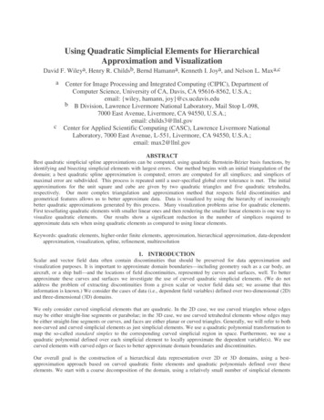
Using Quadratic Simplicial Elements for HierarchicalApproximation and VisualizationDavid F. Wileya, Henry R. Childsb, Bernd Hamanna, Kenneth I. Joya, and Nelson L. Maxa,cacCenter for Image Processing and Integrated Computing (CIPIC), Department ofComputer Science, University of CA, Davis, CA 95616-8562, U.S.A.;email: {wiley, hamann, joy}@cs.ucdavis.edub B Division, Lawrence Livermore National Laboratory, Mail Stop L-098,7000 East Avenue, Livermore, CA 94550, U.S.A.;email: childs3@llnl.govCenter for Applied Scientific Computing (CASC), Lawrence Livermore NationalLaboratory, 7000 East Avenue, L-551, Livermore, CA 94550, U.S.A.;email: max2@llnl.govABSTRACTBest quadratic simplicial spline approximations can be computed, using quadratic Bernstein-Bézier basis functions, byidentifying and bisecting simplicial elements with largest errors. Our method begins with an initial triangulation of thedomain; a best quadratic spline approximation is computed; errors are computed for all simplices; and simplices ofmaximal error are subdivided. This process is repeated until a user-specified global error tolerance is met. The initialapproximations for the unit square and cube are given by two quadratic triangles and five quadratic tetrahedra,respectively. Our more complex triangulation and approximation method that respects field discontinuities andgeometrical features allows us to better approximate data. Data is visualized by using the hierarchy of increasinglybetter quadratic approximations generated by this process. Many visualization problems arise for quadratic elements.First tessellating quadratic elements with smaller linear ones and then rendering the smaller linear elements is one way tovisualize quadratic elements. Our results show a significant reduction in the number of simplices required toapproximate data sets when using quadratic elements as compared to using linear elements.Keywords: quadratic elements, higher-order finite elements, approximation, hierarchical approximation, data-dependentapproximation, visualization, spline, refinement, multiresolution1. INTRODUCTIONScalar and vector field data often contain discontinuities that should be preserved for data approximation andvisualization purposes. It is important to approximate domain boundaries—including geometry such as a car body, anaircraft, or a ship hull—and the locations of field discontinuities, represented by curves and surfaces, well. To betterapproximate these curves and surfaces we investigate the use of curved quadratic simplicial elements. (We do notaddress the problem of extracting discontinuities from a given scalar or vector field data set; we assume that thisinformation is known.) We consider the cases of data (i.e., dependent field variables) defined over two-dimensional (2D)and three-dimensional (3D) domains.We only consider curved simplicial elements that are quadratic. In the 2D case, we use curved triangles whose edgesmay be either straight-line segments or parabolae; in the 3D case, we use curved tetrahedral elements whose edges maybe either straight-line segments or curves, and faces are either planar or curved triangles. Generally, we will refer to bothnon-curved and curved simplicial elements as just simplicial elements. We use a quadratic polynomial transformation tomap the so-called standard simplex to the corresponding curved simplicial region in space. Furthermore, we use aquadratic polynomial defined over each simplicial element to locally approximate the dependent variable(s). We usecurved elements with curved edges or faces to better approximate domain boundaries and discontinuities.Our overall goal is the construction of a hierarchical data representation over 2D or 3D domains, using a bestapproximation approach based on curved quadratic finite elements and quadratic polynomials defined over theseelements. We start with a coarse decomposition of the domain, using a relatively small number of simplicial elements
and placing curved simplices in areas where domain boundaries or field discontinuities occur. We then compute a0(globally) best least squares approximation, a quadratic spline approximation for the dependent variable(s) that is C continuous. The physical loci of discontinuities play the same roles as domain boundaries: Two simplicial elements mayshare the same edge (face)—geometrically—defining the locus of a discontinuity, but the field function defined over thetwo elements is discontinuous along the shared edge (face). We compute local errors for each simplicial element, and webisect a certain percentage of the elements with largest errors, update the simplicial domain decomposition accordingly,and compute a new best quadratic spline approximation. We iterate this process until a specified error condition is met orthe number of simplicial elements exceeds some threshold.Figure 1. Decomposition of domain around awing, using 2D curved quadratic simplices. Thereare two distinct regions in the field defined by thevertices and edges: the region left of thediscontinuity (shaded) and the region right of thediscontinuity. (The bullets and circles indicate thesix polynomial coefficients associated with eachelement.)Our approach belongs to the class of refinement methods. These methods are based on the principle of refiningintermediate data approximations by inserting additional points or elements until a certain termination criterion issatisfied. We have developed our method with a focus on the needs of massive scientific data visualization, see 6. Toenable interactive visualization of massive data, it is possible to use either low-resolution best approximationseverywhere or to adaptively “insert” high-resolution approximations locally into an otherwise relatively coarseapproximation. Our approximation algorithm is based on these steps: Initial simplicial domain decomposition. Assuming that either a polygonal (polyhedral) or an analyticaldefinition is known for all boundaries and field discontinuities, we construct a coarse simplicialdecomposition of this domain. We use curved edges (faces) in areas where they are needed to betterapproximate curved boundaries or discontinuities. (The quadratic transformations, mapping the standardsimplex defined in so-called parameter space to deformed simplices in so-called physical space, aredefined by specifying corresponding point pairs in the two spaces such that one obtains a one-to-one,bijective mapping.) Figure 1 shows a possible initial simplicial decomposition of space around a wing crosssection.Best approximation. In the 2D case, each simplicial element has six associated knots (having specificlocations in the domain and associated coefficients), one knot per corner and one knot per edge. Six knotsin parameter space are associated with six points in physical space, and this association defines the neededquadratic mapping for a simplex. (Accordingly, the number of knots is ten in the 3D case.) For simplicity,we consider only knots that are uniformly distributed along the edges of the standard simplex. We associatea quadratic polynomial with each simplicial element, which approximates the dependent variable(s) overthe corresponding region in space. We represent each quadratic basis polynomial in so-called BernsteinBézier form, see 4. Assuming that the function to be approximated is known in analytical form, it is possibleto compute the unique best quadratic spline approximation defined as a linear combination of the quadraticbasis functions. The best approximation, understood in a least squares sense, is the result of solving thenormal equations, see 3.
Adaptive bisection. We compute an error value for each simplicial element once a best approximation iscomputed. We use the L2 norm to compute simplex-specific error values. The set of simplices is orderedaccording to the simplex-specific error values. To compute a next-level best quadratic approximation wedetermine a certain percentage of simplices with largest error values and bisect them by splitting them atthe midpoint of their longest edge. If a simplex's longest edge is not unique, we choose the edge to be splitrandomly. In the case of curved edges, we use arc length to determine the longest edge to be bisected.Splitting a simplex into two simplices induces additional splits for all those simplices that share the splitedge. We update a simplicial domain decomposition by considering all edge bisections and compute a newbest approximation. We repeat the process of identifying simplices with largest errors, bisecting thesesimplices, and computing a new best approximation until we obtain an approximation for which the largestsimplex-specific error is below a certain error threshold or until a maximal number of simplices is reached.Hierarchical data representation. To support level-of-detail visualization we can store multiple bestapproximations of different resolutions. For each best approximation, we need to store the polynomialcoefficients of each simplicial element—for its shape and the field defined over it. Considering a noncurved simplicial element, we only need to store its three (four) corner points and the coefficients of thefield defined over the element. Considering a curved element, we need to store all polynomial coefficientsdefining the shape of the element, in addition to the coefficients of the quadratic polynomial defining thefield over the element. We store a fixed number of best approximations such that either the number ofsimplices increases in a specified fashion or the maximal simplex-specific error decreases in a certain wayfrom one resolution to the next.2. PREVIOUS WORKRelated work in the areas of hierarchical data representation and visualization is discussed in, for example, 11, 16.Simplification methods are described in 9, 18. Wavelet methods, in general, work well for rectilinear 2D and 3D grids andare described in 2, 14. Refinement methods, similar to our method, are described in 7, 8. Data-dependent triangulationschemes, i.e., schemes concerned with the construction of approximations using near-optimally shaped and placedsimplicial elements, are described in 13. Our method is also a grid generation method, and references for this area are 10,17. Finite element methods are discussed in 19.3. MAPPING THE STANDARD SIMPLEXIn the 2D case, the standard simplex in parameters space is the triangle with corners (0, 0), (1, 0), and (0, 1). Weassociate a 2D quadratic Bernstein-Bézier polynomialBi2, j (u, v ) Bi2, j (u, v ) , defined as2!(1 u v ) 2 i j ui v j , i, j 0, i j 2 ,(2 i j )! i! j!(1)with each corner and midpoint of each edge. The six basis polynomials correspond to the six knotsu i , j (ui , j , vi , j ) (2i , 2j ), i, j 0, i j 2 in parameter space, see Figure 2. We map the standard triangle to aFigure 2. Correspondence between 2D basis functionscircles) inuv -parameter space.Bi2, jin “index” space and knots (indicated by bullets and
curved triangular region in physical space by mapping the six knotsu i, j in parameter space to six corresponding pointsx i , j (xi , j , yi , j ) in physical space, using a quadratic mapping. The quadratic mapping is defined asx(u ) x (u, v )y (u, v )bi , j Bi2, j (u) ci , j Bi2, j (u, v )i, ji, jdi , j Bi2, j (u, v ), i, j 0, i j 2 .(2)i, jThe mapping between parameter and physical space must be one-to-one. Figure 3 depicts a general mapping of thestandard triangle in uv -parameter space to a curved triangle in xy -physical space.Figure 3. Correspondence betweenuv -parameter space and xy -physical space.In the 3D case, the standard simplex is the tetrahedron with corners (0, 0, 0), (1, 0, 0), (0, 1, 0), and (0, 0, 1). Weassociate a 3D quadratic Bernstein-Bézier polynomialBi2, j , k (u, v, w) Bi2, j ,k (u, v, w) , defined as2!(1 u v w) 2 i j k ui v j wk , i, j, k 0, i j k 2 ,(2 i j k )! i! j! k!(3)with each corner and midpoint of each edge. The ten basis polynomials correspond to the ten knotsui , j , k (ui , j , k , vi , j , k , wi , j , k ) ( , , ), i, j, k 0, i j k 2i2j2k2in parameter space. We map the standardtetrahedron to a curved tetrahedral region in physical space by mapping the ten knotscorresponding pointsu i , j ,k in parameter space to tenx i , j , k (xi , j .k , yi , j , k , zi , j , k ) in physical space, using a quadratic mapping. The quadraticmapping, in the 3D case, can be extended from 2. Figure 4 depicts the mapping of the standard tetrahedron in parameterspace to a curved tetrahedron in physical space.Figure 4. Mapping of standard tetrahedron in parameter space to curved tetrahedron in physical space.
4. INITIAL DOMAIN DECOMPOSITIONThe main objective driving the development of our method is to construct a hierarchical representation of very largescientific data, where real-time and adaptive data visualization is crucial. Data sets resulting from computationalsimulations are typically defined on a grid, and the dependent variables are associated with either the vertices (alsocalled nodes) or the elements defining the grid. Either of these types of data can be approximated by our method. Theoriginal grid, its boundaries, and possibly known locations of field discontinuities (in the dependent field variables)influence how we define an initial simplicial decomposition of the domain.The objective is to initially represent the domain with a relatively small number of (curved) simplicial elements, usingcurved elements where they help to better approximate domain boundaries and (known) field discontinuities. We assumethat we are provided with data representing field discontinuities and the domain boundary. This data is specified as a setof points and their connectivity. In the 2D case, the connectivity information defines linear splines. In the 3D case, theconnectivity information defines linear spline (triangular) surfaces. Figure 5 shows a sample input and one desirableinitial domain decomposition.Figure 5. Sample input specification (left) and possible initial decomposition (right) utilizing curved (shaded) andnon-curved simplices. Input points are shown as solid black squares; many points are used to represent the linearspline along the discontinuity between the dark-gray and light-gray regions (left image) and along the wingboundary. Bullets and circles represent corner and edge vertices of the elements in the initial decomposition.We construct an initial decomposition by performing this sequence of steps: First, we classify the points; next, wedetermine connected paths; subsequently, we determine region boundaries; then, we determine a region hierarchy; next,we fit quadratic curves to the paths; and, finally, we triangulate (tetrahedralize) the regions. We describe these steps inmore detail for the 2D case:1) Point classification. We classify a point as detached, hanging, normal, or junction if it is connected to zero, one,two, or more than two edges, respectively. Detached points are considered extraneous and are ignored through therest of the region identification process.2) Path determination. In this step, the goal is to find the set of paths in the input data, where a path is defined as asequence of two or more points beginning and ending with hanging or junction points and containing any number ofnormal points in-between. A loop path is a path beginning and ending with the same point—having at least onenormal point in-between. To determine the paths, we first mark all the edges such that it is possible to determine if ithas been traversed. Then, we select a seed edge at random and consider one of the endpoints; if the consideredendpoint is normal, we traverse to the neighboring edge. We continue this traversal until the neighboring edge hasalready been traversed (forming a loop) or the edge’s endpoint is classified as hanging or junction. If a loop pathcannot be formed, we continue traversing in the opposite direction by considering the second endpoint of the seededge. We then select a non-traversed edge at random and perform the same traversal. All paths are determined whenall edges have been traversed. Figure 6 shows a sample classification and illustrates edge traversal.
Figure 6. Point classification and path determination. Points areclassified as detached (D), hanging (H), normal (N), and junction(J). There are three paths in this example, defined by the three edgesequences 0123, 4, and 8567.3) Determination of region boundaries. In this step, we find the paths that bound the various regions. In general, aregion is bounded by a sequence of paths, but, it is possible to have non-closed regions, which we call crackregions. We select a seed path at random and traverse the path in an arbitrary direction. If the endpoint in thedirection we traverse is a junction, we make a right-hand turn—and consider all the paths that connect to thisendpoint and select the path that contains the edge that most closely represents a right-hand turn by considering theincident angles. We repeatedly make right-hand turns until the seed path is reached. Then, we traverse the seed pathin the same direction, making left-hand turns at junctions. These two traversals, in general, yield two distinct regionboundaries. It is possible to trace the same region boundary twice; if this is the case, we discard one of the results. Acrack region is formed when the resulting sequence of paths is not closed, i.e., when the seed path cannot be reachedby only traversing the obtained sequence either forward or backward. If a hanging point is encountered duringtraversal, we perform a U turn and continue the traversal over the already traversed path(s). Once a not-yet-traversedpath is reached, we “cut off” the sequence of paths that was traversed twice, forming a crack region. We thencontinue normal traversal, but, due to a possible U turn, we may encounter already traversed paths. When this is thecase, we form additional crack regions by applying a cut-off step when a non-traversed path is reached. We musttake special care when the traversal returns to a path that has already been traversed. This case leads to the formationof an island region. In this case, a closed region is formed, and we cut off the sequence that defines the island andcontinue traversal. Figure 7 shows an example.Figure 7. Region boundary construction. Points are classified as hanging (black), normal (gray), and junction(blue). Edges are labeled according to the path to which they belong. Blue paths (6, 7, 8, 9, and 10) denote closedregion boundaries. Orange paths (0, 1, 2, 3, and 5) indicate crack regions. The green path (4) indicates an islandregion. The regions are defined by path sequences 0, 1-2-3, 4, 5, 6-10-9-8, and 6-7.4) Determination of region hierarchy. To determine which regions are inside other regions, we sort the regions basedon size of their bounding boxes. Starting with the minimum-area region, we iteratively test whether any non-sharedpoint is contained in the next-larger-area region. If this is not the case, then we proceed to the next-larger-arearegion, etc. Once we have found a containing (parent) region, we add the smaller region as a child to the parent.5) Fitting curves to paths. We fit quadratic curves to the paths by finding sequences of points that curve in the samedirection. (We limit the angle by which a sequence of points can curve, to prevent “spiral” cases.) Points that are colinear are fitted exactly by a quadratic curve. To preserve the polygonal domain boundary exactly, boundary pathsare not approximated. Quadratic curves are fitted to points using least squares approximation. We perform theapproximation relative to the axis formed by the endpoints of a sequence. For simplicity, we only consider quadratic
curves whose three control points are located at the endpoints and at the midpoint of the axis. Error is determined bythe L2 norm of the distance between the fitted curve and th
Related work in the areas of hierarchical data representation and visualization is discussed in, for example, 11, 16. Simplification methods are described in 9, 18. Wavelet methods, in general, work well for rectilinear 2D and 3D grids and are described in 2, 14. Refinement methods, similar to our method, a