WIXLIB

826Chapter Nineteen Linear Programmingx1 the quantity of product 1. Generally, decision variables have profits, costs, times, or asimilar measure of value associated with them. Knowing this can help you identify the decision variables in a problem.Constraints are restrictions or requirements on one or more decision variables, and theyrefer to available amounts of resources such as labor, material, or machine time, or to minimalrequirements, such as “Make at least 10 units of product 1.” It can be helpful to give a nameto each constraint, such as “labor” or “material 1.” Let’s consider some of the different kindsof constraints you will encounter.1. A constraint that refers to one or more decision variables. This is the most common kindof constraint. The constraints in Example 1 are of this type.2. A constraint that specifies a ratio. For example, “The ratio of x1 to x2 must be at least 3to 2.” To formulate this, begin by setting up the following ratio:x13 x22Then, cross multiply, obtaining2x1 3x2This is not yet in a suitable form because all variables in a constraint must be on the left-handside of the inequality (or equality) sign, leaving only a constant on the right-hand side. Toachieve this, we must subtract the variable amount that is on the right side from both sides.That yields2x1 3x2 0(Note that the direction of the inequality remains the same.)3. A constraint that specifies a percentage for one or more variables relative to one or moreother variables. For example, “x1 cannot be more than 20 percent of the mix.” Suppose thatthe mix consists of variables x1, x2, and x3. In mathematical terms, this would bex1 .20(x1 x2 x3)As always, all variables must appear on the left-hand side of the relationship. To accomplishthat, we can expand the right-hand side, and then subtract the result from both sides. Expanding yieldsx1 .20x1 .20x2 .20x3Subtracting yields.80x1 .20x2 .20x3 0Once you have formulated a model, the next task is to solve it. The following sectionsdescribe two approaches to problem solution: graphical solutions and computer solutions.19.3 GRAPHICAL LINEAR PROGRAMMINGLO19.3 Solve simplelinear programming problems using the graphicalmethod.Graphical linear programmingGraphical method for findingoptimal solutions to twovariable problems.Graphical linear programming is a method for finding optimal solutions to two-variableproblems. This section describes that approach.Outline of Graphical ProcedureThe graphical method of linear programming involves plotting the constraint lines on a graphand identifying an area on the graph that satisfies all of the constraints. The area is referred toas the feasible solution space. Next, the objective function is plotted and used to identify theoptimal point in the feasible solution space. The coordinates of the point can sometimes beread directly from the graph, although generally an algebraic determination of the coordinatesof the point is necessary.

827Chapter Nineteen Linear ProgrammingThe general procedure followed in the graphical approach is as follows:1.2.3.4.5.Set up the objective function and the constraints in mathematical format.Plot the constraints.Identify the feasible solution space.Plot the objective function.Determine the optimum solution.The technique can best be illustrated through solution of a typical problem. Consider theproblem described in Example 2.Graphing the Problem and Finding the Optimal SolutionGeneral description: A firm that assembles computers and computer equipment is aboutto start production of two new types of microcomputers. Each type will require assemblytime, inspection time, and storage space. The amounts of each of these resources that can bedevoted to the production of the microcomputers is limited. The manager of the firm wouldlike to determine the quantity of each microcomputer to produce in order to maximize theprofit generated by sales of these microcomputers.Additional information: In order to develop a suitable model of the problem, the managerhas met with design and production personnel. As a result of those meetings, the managerhas obtained the following information.Profit per unitAssembly time per unitInspection time per unitStorage space per unitType 1Type 2 604 hours2 hours3 cubic feet 5010 hours1 hour3 cubic feetThe manager also has acquired information on the availability of company resources.These (daily) amounts are as follows.ResourceAmount AvailableAssembly timeInspection timeStorage space100 hours22 hours39 cubic feetThe manager met with the firm’s marketing manager and learned that demand for themicrocomputers was such that whatever combination of these two types of microcomputersis produced, all of the output can be sold.In terms of meeting the assumptions, it would appear that the relationships are linear: Thecontribution to profit per unit of each type of computer and the time and storage space perunit of each type of computer are the same regardless of the quantity produced. Therefore, thetotal impact of each type of computer on the profit and each constraint is a linear function ofthe quantity of that variable. There may be a question of divisibility because, presumably, onlywhole units of computers will be sold. However, because this is a recurring process (i.e., thecomputers will be produced daily; a noninteger solution such as 3.5 computers per day willresult in 7 computers every other day), this does not seem to pose a problem. The question ofcertainty cannot be explored here; in practice, the manager could be questioned to determineif there are any other possible constraints and whether the values shown for assembly times,and so forth, are known with certainty. For the purposes of discussion, we will assume certainty. Last, the assumption of nonnegativity seems justified; negative values for productionquantities would not make sense.EXAMPLE2

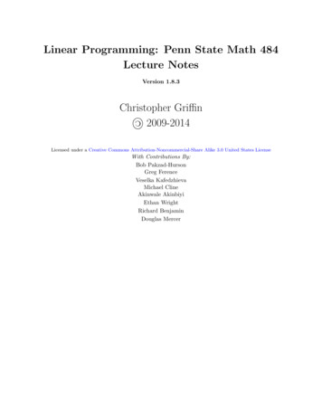
828Chapter Nineteen Linear ProgrammingBecause we have concluded that linear programming is appropriate, let us now turn our attentionto constructing a model of the microcomputer problem. First, we must define the decision variables.Based on the statement “The manager . . . would like to determine the quantity of each microcomputer to produce,” the decision variables are the quantities of each type of computer. Thus,x1 quantity of type 1 to producex2 quantity of type 2 to produceNext, we can formulate the objective function. The profit per unit of type 1 is listed as 60,and the profit per unit of type 2 is listed as 50, so the appropriate objective function isMaximize Z 60x1 50x2where Z is the value of the objective function, given values of x1 and x2. Theoretically, amathematical function requires such a variable for completeness. However, in practice, theobjective function often is written without the Z as sort of a shorthand version. (That approachis underscored by the fact that computer input does not call for Z: It is understood. The outputof a computerized model does include a Z, though.)Now for the constraints. There are three resources with limited availability: assembly time,inspection time, and storage space. The fact that availability is limited means that these constraints will all be constraints. Suppose we begin with the assembly constraint. The type 1microcomputer requires 4 hours of assembly time per unit, whereas the type 2 microcomputerrequires 10 hours of assembly time per unit. Therefore, with a limit of 100 hours available, theassembly constraint is4x1 10x2 100 hoursSimilarly, each unit of type 1 requires 2 hours of inspection time, and each unit of type 2requires 1 hour of inspection time. With 22 hours available, the inspection constraint is2x1 1x2 22(Note: The coefficient of 1 for x2 need not be shown. Thus, an alternative form for this constraint is 2x1 x2 22.) The storage constraint is determined in a similar manner:3x1 3x2 39There are no other system or individual constraints. The nonnegativity constraints arex1, x2 0In summary, the mathematical model of the microcomputer problem isx1 quantity of type 1 to producex2 quantity of type 2 to produceMaximize 60x1 50x2Subject toAssemblyInspectionStorage4x1 10x22x1 1x23x1 3x2x1, x2 100 hours 22 hours 39 cubic feet 0The next step is to plot the constraints.Plotting ConstraintsBegin by placing the nonnegativity constraints on a graph, as in Figure 19.1. The procedurefor plotting the other constraints is simple:1.Replace the inequality sign with an equal sign. This transforms the constraint into anequation of a straight line.

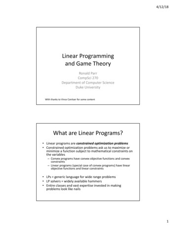
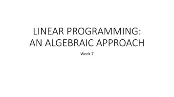
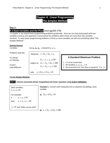
Chapter Nineteen829Linear Programmingx2FIGURE 19.1Quantity of type 2Graph showing thenonnegativity constraintsArea offeasibilityx1 0Nonnegativityconstraintsx2 0x10Quantity of type 12.3.4.5.Determine where the line intersects each axis.a. To find where it crosses the x2 axis, set x1 equal to zero and solve the equation for thevalue of x2.b. To find where it crosses the x1 axis, set x2 equal to zero and solve the equation for thevalue of x1Mark these intersections on the axes, and connect them with a straight line. (Note: If aconstraint has only one variable, it will be a vertical line on a graph if the variable is x1,or a horizontal line if the variable is x2.)Indicate by shading (or by arrows at the ends of the constraint line) whether the inequality is greater than or less than. (A general rule to determine which side of the line satisfies the inequality is to pick a point that is not on line, such as 0,0, solve the equationusing these values, and see whether it is greater than or less than the constraint amount.)Repeat steps 1–4 for each constraint.Consider the assembly time constraint:4x1 10x2 100Removing the inequality portion of the constraint produces this straight line:4x1 10x2 100Next, identify the points where the line intersects each axis, as step 2 describes. Thus withx2 0, we find4x1 10(0) 100Solving, we find that 4x1 100, so x1 25 when x2 0. Similarly, we can solve the equationfor x2 when x1 0:4(0) 10x2 100Solving for x2, we find x2 10 when x1 0.Thus, we have two points: x1 0, x2 10, and x1 25, x2 0. We can now add this line toour graph of the nonnegativity constraints by connecting these two points (see Figure 19.2).Next we must determine which side of the line represents points that are less than 100. To dothis, we can select a test point that is not on the line, and we can substitute the x1 and x2 values of thatpoint into the left-hand side of the equation of the line. If the result is less than 100, this tells us thatall points on that side of the line are less than the value of the line (e.g., 100). Conversely, if the resultis greater than 100, this indicates that the other side of the line represents the set of points that willyield values that are less than 100. A relatively simple test point to use is the origin (i.e., x1 0, x2 0). Substituting these values into the equation yields obviously this is less than 100. Hence, theside of the line closest to the origin represents the “less than” area (i.e., the feasible region).4(0) 10(0) 0

830Chapter Nineteen Linear ProgrammingFIGURE 19.2 Plot of the first constraintFIGURE 19.3 The feasible region, given(assembly time)the first constraint and thenonnegativity constraintsx2x210104x1 10Assemx 2 100Feasibleregion025x1blytime025x1The feasible region for this constraint and the nonnegativity constraints then becomes theshaded portion shown in Figure 19.3.For the sake of illustration, suppose we try one other point, say x1 10, x2 10. Substituting these values into the assembly constraint yields4(10) 10(10) 140Clearly this is greater than 100. Therefore, all points on this side of the line are greater than100 (see Figure 19.4).Continuing with the problem, we can add the two remaining constraints to the graph. Forthe inspection constraint:1.Convert the constraint into the equation of a straight line by replacing the inequality signwith an equality sign:2x1 1x2 22 becomes 2x1 1x2 222.Set x1 equal to zero and solve for x2:2(0) 1x2 22Solving, we find x2 22. Thus, the line will intersect the x2 axis at 22.3.Next, set x2 equal to zero and solve for x1:2x1 1(0) 22Solving, we find x1 11. Thus, the other end of the line will intersect the x1 axis at 11.4.Add the line to the graph (see Figure 19.5).Note that the area of feasibility for this constraint is below the line (Figure 19.5). Again thearea of feasibility at this point is shaded in for illustration, although when graphing problems,it is more practical to refrain from shading in the feasible region until all constraint lines havebeen drawn. However, because constraints are plotted one at a time, using a small arrow at theend of each constraint to indicate the direction of feasibility can be helpful.The storage constraint is handled in the same manner:1.Convert it into an equality:3x1 3x2 392.Set x1 equal to zero and solve for x2:3(0) 3x2 39

831Chapter Nineteen Linear ProgrammingFIGURE 19.5 Partially completed graph, showingFIGURE 19.4 The point (10, 10) is abovethe assembly, inspection, andnonnegativity constraintsthe constraint linex2x222Insnctiope (10,10)104x1 10Feasible for inspectionbut not for assemblyFeasible for assemblybut not for inspection10x 2 100AssFeasible forboth assemblyand inspection100x1250em11bly25x1Solving, x2 13. Thus, x2 13 when x1 0.3.Set x2 equal to zero and solve for x1:3x1 3(0) 39Solving, x1 13. Thus, x1 13 when x2 0.4.Add the line to the graph (see Figure 19.6).Identifying the Feasible Solution SpaceThe feasible solution space is the set of all points that satisfies all constraints. (Recall that thex1 and x2 axes form nonnegativity constraints.) The heavily shaded area shown in Figure 19.6is the feasible solution space for our problem.The next step is to determine which point in the feasible solution space will producethe optimal value of the objective function. This determination is made using the objectivefunction.Plotting the Objective Function LinePlotting an objective function line involves the same logic as plotting a constraint line: Determine where the line intersects each axis. Recall that the objective function for the microcomputer problem is60x1 50x2FIGURE 19.622Completed graph of themicrocomputer problemshowing all constraints andthe feasible solution Assem1113bly25x1

832Chapter Nineteen Linear ProgrammingThis is not an equation because it does not include an equal sign. We can get around this bysimply setting it equal to some quantity. Any quantity will do, although one that is evenlydivisible by both coefficients is desirable.Suppose we decide to set the objective function equal to 300. That is,60x1 50x2 300We can now plot the line on our graph. As before, we can determine the x1 and x2 interceptsof the line by setting one of the two variables equal to zero, solving for the other, and thenreversing the process. Thus, with x1 0, we have60(0) 50x2 300Solving, we find x2 6. Similarly, with x2 0, we have60x1 50(0) 300Solving, we find x1 5. This line is plotted in Figure 19.7.The profit line can be interpreted in the following way: It is an isoprofit line; every pointon the line (i.e., every combination of x1 and x2 that lies on the line) will provide a profit of 300. We can see from the graph many combinations that are both on the 300 profit line andwithin the feasible solution space. In fact, considering noninteger as well as integer solutions,the possibilities are infinite.Suppose we now consider another line, say the 600 line. To do this, we set the objectivefunction equal to this amount. Thus,60x1 50x2 600Solving for the x1 and x2 intercepts yields these two points:x1 interceptx2 interceptx1 10x1 0x2 0x2 12This line is plotted in Figure 19.8, along with the previous 300 line for purposes ofcomparison.Two things are evident in Figure 19.8 regarding the profit lines. One is that the 600 lineis farther from the origin than the 300 line; the other is that the two lines are parallel. Thelines are parallel because they both have the same slope. The slope is not affected by the rightside of the equation. Rather, it is determined solely by the coefficients 60 and 50. It wouldFIGURE 19.7 Microcomputer problem withFIGURE 19.8 Microcomputer problem with 300 profit line addedprofit lines of 300 and 600x2x22222pepeInsInsne00 6t ofi 300 13Assfitbly011Pr30 325x105em10 1113bly25x1

833Chapter Nineteen Linear Programmingbe correct to conclude that regardless of the quantity we select for the value of the objectivefunction, the resulting line will be parallel to these two lines. Moreover, if the amount isgreater than 600, the line will be even farther away from the origin than the 600 line. If thevalue is less than 300, the line will be closer to the origin than the 300 line. And if the valueis between 300 and 600, the line will fall between the 300 and 600 lines. This knowledgewill help in determining the optimal solution.Consider a third line, one with the profit equal to 900. Figure 19.9 shows that line alongwith the previous two profit lines. As expected, it is parallel to the other two, and even fartheraway from the origin. However, the line does not touch the feasible solution space at all. Consequently, there is no feasible combination of x1 and x2 that will yield that amount of profit.Evidently, the maximum possible profit is an amount between 600 and 900, which we cansee by referring to Figure 19.9. We could continue to select profit lines in this manner, andeventually, we could determine an amount that would yield the greatest profit. However, thereis a much simpler alternative. We can plot just one line, say the 300 line. We know that allother lines will be parallel to it. Consequently, by moving this one line parallel to itself we can“test” other profit lines. We also know that as we move away from the origin, the profits getlarger. What we want to know is how far the line can be moved out from the origin and still betouching the feasible solution space, and the values of the decision variables at that point ofgreatest profit (i.e., the optimal solution). Locate this point on the graph by placing a straightedge along the 300 line (or any other convenient line) and sliding it away from the origin,being careful to keep it parallel to the line. This approach is illustrated in Figure 19.10.Once we have determined where the optimal solution is in the feasible solution space, wemust determine the values of the decision variables at that point. Then, we can use that information to compute the profit for that combination.Note that the optimal solution is at the intersection of the inspection boundary and the storage boundary (see Figure 19.10). In other words, the optimal combination of x1 and x2 mustsatisfy both boundary (equality) conditions. We can determine those values by solving thetwo equations simultaneously. The equations are:Inspection2x1 1x2 22Storage3x1 3x2 39The idea behind solving two simultaneous equations is to algebraically eliminate one of theunknown variables (i.e., to obtain an equation with a single unknown). This can be accomplished by multiplying the constants of one of the equations by a fixed amount and thenadding (or subtracting) the modified equation from the other. (Occasionally, it is easier tomultiply each equation by a fixed quantity.) For example, we can eliminate x2 by multiplyingFIGURE 19.9 Microcomputer problemFIGURE 19.10 Finding the optimalwith profit lines of 300, 600, and 900solution to the

side of the inequality (or equality) sign, leaving only a constant on the right-hand side. To achieve this, we must subtract the variable amount that is on the right side from both sides. That yields 2 x 1 3 x 2 0 (Note that the direction of the inequality remains the same.) 3. A c