Transcription
FUNDAMENTALS OF SAMPLED DATA SYSTEMSANALOG-DIGITAL CONVERSION1. Data Converter History2. Fundamentals of Sampled Data Systems2.12.22.32.42.5Coding and QuantizingSampling TheoryData Converter AC ErrorsGeneral Data Converter SpecificationsDefining the Specifications3. Data Converter Architectures4. Data Converter Process Technology5. Testing Data Converters6. Interfacing to Data Converters7. Data Converter Support Circuits8. Data Converter Applications9. Hardware Design TechniquesI. Index
ANALOG-DIGITAL CONVERSION
FUNDAMENTALS OF SAMPLED DATA SYSTEMS2.1 CODING AND QUANTIZINGCHAPTER 2FUNDAMENTALS OF SAMPLED DATASYSTEMSSECTION 2.1: CODING AND QUANTIZINGWalt Kester, Dan Sheingold, James BryantAnalog-to-digital converters (ADCs) translate analog quantities, which arecharacteristic of most phenomena in the "real world," to digital language, used ininformation processing, computing, data transmission, and control systems. Digital-toanalog converters (DACs) are used in transforming transmitted or stored data, or theresults of digital processing, back to "real-world" variables for control, informationdisplay, or further analog processing. The relationships between inputs and outputs ofDACs and ADCs are shown in Figure 2.1.VREFMSBDIGITALINPUTN-BITS FSN-BITDACANALOGOUTPUTLSBRANGE(SPAN)0 OR –FSVREFMSB FSRANGE(SPAN)0 OR re 2.1: Digital-to-Analog Converter (DAC) and Analog-to-Digital Converter(ADC) Input and Output DefinitionsAnalog input variables, whatever their origin, are most frequently converted bytransducers into voltages or currents. These electrical quantities may appear (1) as fast orslow "dc" continuous direct measurements of a phenomenon in the time domain, (2) asmodulated ac waveforms (using a wide variety of modulation techniques), (3) or in somecombination, with a spatial configuration of related variables to represent shaft angles.2.1
ANALOG-DIGITAL CONVERSIONExamples of the first are outputs of thermocouples, potentiometers on dc references, andanalog computing circuitry; of the second, "chopped" optical measurements, ac straingage or bridge outputs, and digital signals buried in noise; and of the third, synchros andresolvers.The analog variables to be dealt with in this chapter are those involving voltages orcurrents representing the actual analog phenomena. They may be either wideband ornarrowband. They may be either scaled from the direct measurement, or subjected tosome form of analog pre-processing, such as linearization, combination, demodulation,filtering, sample-hold, etc.As part of the process, the voltages and currents are "normalized" to ranges compatiblewith assigned ADC input ranges. Analog output voltages or currents from DACs aredirect and in normalized form, but they may be subsequently post-processed (e.g., scaled,filtered, amplified, etc.).Information in digital form is normally represented by arbitrarily fixed voltage levelsreferred to "ground," either occurring at the outputs of logic gates, or applied to theirinputs. The digital numbers used are all basically binary; that is, each "bit," or unit ofinformation has one of two possible states. These states are "off," "false," or "0," and"on," "true," or "1." It is also possible to represent the two logic states by two differentlevels of current, however this is much less popular than using voltages. There is also noparticular reason why the voltages need be referenced to ground—as in the case ofemitter-coupled-logic (ECL), positive-emitter-coupled-logic (PECL) or low-voltagedifferential-signaling logic (LVDS) for example.Words are groups of levels representing digital numbers; the levels may appearsimultaneously in parallel, on a bus or groups of gate inputs or outputs, serially (or in atime sequence) on a single line, or as a sequence of parallel bytes (i.e., "byte-serial") ornibbles (small bytes). For example, a 16-bit word may occupy the 16 bits of a 16-bit bus,or it may be divided into two sequential bytes for an 8-bit bus, or four 4-bit nibbles for a4-bit bus.Although there are several systems of logic, the most widely used choice of levels arethose used in TTL (transistor-transistor logic) and, in which positive true, or 1,corresponds to a minimum output level of 2.4 V (inputs respond unequivocally to "1"for levels greater than 2.0 V); and false, or 0, corresponds to a maximum output level of 0.4 V (inputs respond unequivocally to "0" for anything less than 0.8 V). It should benoted that even though CMOS is more popular today than TTL, CMOS logic levels aregenerally made to be compatible with the older TTL logic standard.A unique parallel or serial grouping of digital levels, or a number, or code, is assigned toeach analog level which is quantized (i.e., represents a unique portion of the analogrange). A typical digital code would be this array:a7 a6 a5 a4 a3 a2 a1 a0 1 0 1 1 1 0 0 1It is composed of eight bits. The "1" at the extreme left is called the "most significant bit"(MSB, or Bit 1), and the one at the right is called the "least significant bit" (LSB, or2.2
FUNDAMENTALS OF SAMPLED DATA SYSTEMS2.1 CODING AND QUANTIZINGbit N: 8 in this case). The meaning of the code, as either a number, a character, or arepresentation of an analog variable, is unknown until the code and the conversionrelationship have been defined. It is important not to confuse the designation of aparticular bit (i.e., Bit 1, Bit 2, etc.) with the subscripts associated with the "a" array. Thesubscripts correspond to the power of 2 associated with the weight of a particular bit inthe sequence.The best-known code (other than base 10) is natural or straight binary (base 2). Binarycodes are most familiar in representing integers; i.e., in a natural binary integer codehaving N bits, the LSB has a weight of 20 (i.e., 1), the next bit has a weight of 21 (i.e., 2),and so on up to the MSB, which has a weight of 2N–1 (i.e., 2N/2). The value of a binarynumber is obtained by adding up the weights of all non-zero bits. When the weighted bitsare added up, they form a unique number having any value from 0 to 2N – 1. Eachadditional trailing zero bit, if present, essentially doubles the size of the number.In converter technology, full-scale (abbreviated FS) is independent of the number of bitsof resolution, N. A more useful coding is fractional binary which is always normalized tofull-scale. Integer binary can be interpreted as fractional binary if all integer values aredivided by 2N. For example, the MSB has a weight of ½ (i.e., 2(N–1)/2N 2–1), the next bithas a weight of ¼ (i.e., 2–2), and so forth down to the LSB, which has a weight of 1/2N(i.e., 2–N). When the weighted bits are added up, they form a number with any of 2Nvalues, from 0 to (1 – 2–N) of full-scale. Additional bits simply provide more finestructure without affecting full-scale range. The relationship between base-10 numbersand binary numbers (base 2) are shown in Figure 2.2 along with examples of each.WHOLE NUMBERS:Number10 aN–12N–1 aN –22N–2 a121 a020MSBLSBExample: 10112 (1 23) (0 22) (1 21) (1 20) 8 0 2 1 1110FRACTIONAL NUMBERS:Number10 aN–12–1 aN–2 2–2 a12–(N–1) a02–NMSBLSBExample: 0.10112 (1 0.5) (0 0.25) (1 0.125) (1 0.0625) 0.5 0 0.125 0.0625 0.687510Figure 2.2: Representing a Base-10 Number with a Binary Number (Base 2)Unipolar CodesIn data conversion systems, the coding method must be related to the analog input range(or span) of an ADC or the analog output range (or span) of a DAC. The simplest case is2.3
ANALOG-DIGITAL CONVERSIONwhen the input to the ADC or the output of the DAC is always a unipolar positive voltage(current outputs are very popular for DAC outputs, much less for ADC inputs). The mostpopular code for this type of signal is straight binary and is shown in Figure 2.3 for a4-bit converter. Notice that there are 16 distinct possible levels, ranging from the allzeros code 0000, to the all-ones code 1111. It is important to note that the analog valuerepresented by the all-ones code is not full-scale (abbreviated FS), but FS – 1 LSB. Thisis a common convention in data conversion notation and applies to both ADCs andDACs. Figure 2.3 gives the base-10 equivalent number, the value of the base-2 binarycode relative to full-scale (FS), and also the corresponding voltage level for each code(assuming a 10 V full-scale converter. The Gray code equivalent is also shown, and willbe discussed shortly.BASE 10NUMBER 15 14 13 12 11 10 9 8 7 6 5 4 3 2 10SCALE FS – 1LSB 15/16 FS 7/8 FS 13/16 FS 3/4 FS 11/16 FS 5/8 FS 9/16 FS 1/2 FS 7/16 FS 3/8 FS 5/16 FS 1/4 FS 3/16 FS 1/8 FS1LSB 1/16 FS0 10V 01100010001100010000Figure 2.3: Unipolar Binary Codes, 4-bit ConverterFigure 2.4 shows the transfer function for an ideal 3-bit DAC with straight binary inputcoding. Notice that the analog output is zero for the all-zeros input code. As the digitalinput code increases, the analog output increases 1 LSB (1/8 scale in this example) percode. The most positive output voltage is 7/8 FS, corresponding to a value equal to FS –1 LSB. The mid-scale output of 1/2 FS is generated when the digital input code is 100.The transfer function of an ideal 3-bit ADC is shown in Figure 2.5. There is a range ofanalog input voltage over which the ADC will produce a given output code; this range isthe quantization uncertainty and is equal to 1 LSB. Note that the width of the transitionregions between adjacent codes is zero for an ideal ADC. In practice, however, there isalways transition noise associated with these levels, and therefore the width is non-zero.It is customary to define the analog input corresponding to a given code by the codecenter which lies halfway between two adjacent transition regions (illustrated by theblack dots in the diagram). This requires that the first transition region occur at ½ LSB.The full-scale analog input voltage is defined by 7/8 FS, (FS – 1 LSB).2.4
FUNDAMENTALS OF SAMPLED DATA SYSTEMS2.1 CODING AND 01010011100101110111DIGITAL INPUT (STRAIGHT BINARY)Figure 2.4: Transfer Function for Ideal Unipolar 3-bit DAC111110DIGITALOUTPUT(STRAIGHTBINARY)1011001 LSB0111/2 LSB01000100001/81/43/81/25/83/47/8FSANALOG INPUTFigure 2.5: Transfer Function for Ideal Unipolar 3-bit ADC2.5
ANALOG-DIGITAL CONVERSIONGray CodeAnother code worth mentioning at this point is the Gray code (or reflective-binary) whichwas invented by Elisha Gray in 1878 (Reference 1) and later re-invented by Frank Grayin 1949 (see Reference 2). The Gray code equivalent of the 4-bit straight binary code isalso shown in Figure 2.3. Although it is rarely used in computer arithmetic, it has someuseful properties which make it attractive to A/D conversion. Notice that in Gray code, asthe number value changes, the transitions from one code to the next involve only one bitat a time. Contrast this to the binary code where all the bits change when making thetransition between 0111 and 1000. Some ADCs make use of it internally and then convertthe Gray code to a binary code for external use.One of the earliest practical ADCs to use the Gray code was a 7-bit, 100 kSPS electronbeam encoder developed by Bell Labs and described in a 1948 reference (Reference 3).The basic electron beam coder concepts are shown in Figure 2.6 for a 4-bit device. Theearly tubes operated in the serial mode (A). The analog signal is first passed through asample-and-hold, and during the "hold" interval, the beam is swept horizontally acrossthe tube. The Y-deflection for a single sweep therefore corresponds to the value of theanalog signal from the sample-and-hold. The shadow mask is coded to produce theproper binary code, depending on the vertical deflection. The code is registered by thecollector, and the bits are generated in serial format. Later tubes used a fan-shaped beam(shown in Figure 2.6B), creating a "flash" converter delivering a parallel output word.X Deflectors(A) SERIAL MODEY DeflectorsShadow MaskCollectorElectron gun(B) PARALLEL MODEY DeflectorsShadow MaskCollectorElectron gunFigure 2.6: The Electron Beam Coder: (A) Serial Mode and (B) Parallelor "Flash" Mode2.6
FUNDAMENTALS OF SAMPLED DATA SYSTEMS2.1 CODING AND QUANTIZINGEarly electron tube coders used a binary-coded shadow mask, and large errors can occurif the beam straddles two adjacent codes and illuminates both of them. The way theseerrors occur is illustrated in Figure 2.7A, where the horizontal line represents the beamsweep at the mid-scale transition point (transition between code 0111 and code 1000).For example, an error in the most significant bit (MSB) produces an error of ½ scale.These errors were minimized by placing fine horizontal sensing wires across theboundaries of each of the quantization levels. If the beam initially fell on one of thewires, a small voltage was added to the vertical deflection voltage which moved the beamaway from the transition region.(A) 4-BIT BINARY CODESHADOW MASK(B) 4-BIT REFLECTED-BINARY CODE(GRAY 1000011001000010000MSBLSBSHADOW 100010001100010000MSBLSBFigure 2.7: Electron Beam Coder Shadow Masks forBinary Code (A) and Gray Code (B)The errors associated with binary shadow masks were eliminated by using a Gray codeshadow mask as shown in Figure 2.7B. As mentioned above, the Gray code has theproperty that adjacent levels differ by only one digit in the corresponding Gray-codedword. Therefore, if there is an error in a bit decision for a particular level, thecorresponding error after conversion to binary code is only one least significant bit(LSB). In the case of mid-scale, note that only the MSB changes. It is interesting to notethat this same phenomenon can occur in modern comparator-based flash converters dueto comparator metastability. With small overdrive, there is a finite probability that theoutput of a comparator will generate the wrong decision in its latched output, producingthe same effect if straight binary decoding techniques are used. In many cases, Graycode, or "pseudo-Gray" codes are used to decode the comparator bank. The Gray codeoutput is then latched, converted to binary, and latched again at the final output.As a historical note, in spite of the many mechanical and electrical problems relating tobeam alignment, electron tube coding technology reached its peak in the mid-l960s withan experimental 9-bit coder capable of 12-MSPS sampling rates (Reference 4). Shortlythereafter, however, advances in all solid-state ADC techniques made the electron tubetechnology obsolete.2.7
ANALOG-DIGITAL CONVERSIONOther examples where Gray code is often used in the conversion process to minimizeerrors are shaft encoders (angle-to-digital) and optical encoders.ADCs which use the Gray code internally almost always convert the Gray code output tobinary for external use. The conversion from Gray-to-binary and binary-to-Gray is easilyaccomplished with the exclusive-or logic function as shown in Figure re 2.8: Binary-to-Gray and Gray-to-Binary ConversionUsing the Exclusive-Or Logic FunctionBipolar CodesIn many systems, it is desirable to represent both positive and negative analog quantitieswith binary codes. Either offset binary, twos complement, ones complement, or signmagnitude codes will accomplish this, but offset binary and twos complement are by farthe most popular. The relationships between these codes for a 4-bit systems is shown inFigure 2.9. Note that the values are scaled for a 5-V full-scale input/output voltagerange.For offset binary, the zero signal value is assigned the code 1000. The sequence of codesis identical to that of straight binary. The only difference between a straight and offsetbinary system is the half-scale offset associated with analog signal. The most negativevalue (–FS 1 LSB) is assigned the code 0001, and the most positive value( FS – 1 LSB) is assigned the code 1111. Note that in order to maintain perfectsymmetry about mid-scale, the all-zeros code (0000) representing negative full-scale(–FS) is not normally used in computation. It can be used to represent a negative offrange condition or simply assigned the value of the 0001 (–FS 1 LSB).2.8
FUNDAMENTALS OF SAMPLED DATA SYSTEMS2.1 CODING AND QUANTIZINGBASE 10NUMBERSCALE 5V FSOFFSETBINARYTWOSCOMP. 7 6 5 4 3 2 10–1–2–3–4–5–6–7–8 FS – 1LSB 7/8 FS 3/4 FS 5/8 FS 1/2 FS 3/8 FS 1/4 FS 1/8 FS0– 1/8 FS– 1/4 FS– 3/8 FS–1/2 FS–5/8 FS–3/4 FS– FS 1LSB –7/8 FS– FS 4.375 3.750 3.125 2.500 1.875 1.250 00NOT NORMALLY USEDIN COMPUTATIONS (SEE TEXT)*0 0–ONESCOMP.0111011001010100001100100001*0 0 0 MAG.0111011001010100001100100001*1 0 0 e 2.9: Bipolar Codes, 4-bit ConverterThe relationship between the offset binary code and the analog output range of a bipolar3-bit DAC is shown in Figure 2.10. The analog output of the DAC is zero for the zerovalue input code 100. The most negative output voltage is generally defined by the 001code (–FS 1 LSB), and the most positive by 111 ( FS – 1 LSB). The output voltage forthe 000 input code is available for use if desired, but makes the output non-symmetricalabout zero and complicates the mathematics.The offset binary output code for a bipolar 3-bit ADC as a function of its analog input isshown in Figure 2.11. Note that zero analog input defines the center of the mid-scalecode 100. As in the case of bipolar DACs, the most negative input voltage is generallydefined by the 001 code (–FS 1 LSB), and the most positive by 111 ( FS – 1 LSB). Asdiscussed above, the 000 output code is available for use if desired, but makes the outputnon-symmetrical about zero and complicates the mathematics.Twos complement is identical to offset binary with the most-significant-bit (MSB)complemented (inverted). This is obviously very easy to accomplish in a data converter,using a simple inverter or taking the complementary output of a "D" flip-flop. Thepopularity of twos complement coding lies in the ease with which mathematicaloperations can be performed in computers and DSPs. Twos complement, for conversionpurposes, consists of a binary code for positive magnitudes (0 sign bit), and the twoscomplement of each positive number to represent its negative. The twos complement isformed arithmetically by complementing the number and adding 1 LSB. For example,–3/8 FS is obtained by taking the twos complement of 3/8 FS. This is done by firstcomplementing 3/8 FS, 0011 obtaining 1100. Adding 1 LSB, we obtain 1101.2.9
ANALOG-DIGITAL CONVERSION FS 3/8 1/4ANALOGOUTPUT 1DIGITAL INPUT (OFFSET BINARY)Figure 2.10: Transfer Function for Ideal Bipolar 3-bit 1000–FS–3/8–1/4–1/80 1/8 1/4 3/8 FSANALOG INPUTFigure 2.11: Transfer Function for Ideal Bipolar 3-bit ADC2.10
FUNDAMENTALS OF SAMPLED DATA SYSTEMS2.1 CODING AND QUANTIZINGTwos complement makes subtraction easy. For example, to subtract 3/8 FS from 4/8 FS,add 4/8 to –3/8, or 0100 to 1101. The result is 0001, or 1/8, disregarding the extra carry.Ones complement can also be used to represent negative numbers, although it is muchless popular than twos complement and rarely used today. The ones complement isobtained by simply complementing all of a positive number's digits. For instance, theones complement of 3/8 FS (0011) is 1100. A ones complemented code can be formed bycomplementing each positive value to obtain its corresponding negative value. Thisincludes zero, which is then represented by either of two codes, 0000 (referred to as 0 )or 1111 (referred to as 0–). This ambiguity must be dealt with mathematically, andpresents obvious problems relating to ADCs and DACs for which there is a single codewhich represents zero.Sign-magnitude would appear to be the most straightforward way of expressing signedanalog quantities digitally. Simply determine the code appropriate for the magnitude andadd a polarity bit. Sign-magnitude BCD is popular in bipolar digital voltmeters, but hasthe problem of two allowable codes for zero. It is therefore unpopular for mostapplications involving ADCs or DACs.Figure 2.12 summarizes the relationships between the various bipolar codes: offsetbinary, twos complement, ones complement, and sign-magnitude and shows how toconvert between them.To Convert FromToSign Magnitude2's ComplementSign MagnitudeNoChangeIf MSB 1,complementother bits,add 00 012's ComplementIf MSB 1,complementother bits,add 00 01NoChangeOffset binaryComplement MSBIf new MSB 0complementother bits,add 00 01ComplementMSB1's ComplementIf MSB 1,complementother bitsIf MSB 1,add 11 11Offset BinaryComplement MSBIf new MSB 1,complementother bits,add 00 01ComplementMSBNoChange1's ComplementIf MSB 1,complementother bitsIf MSB 1,add 00 01Complement MSBIf new MSB 0,add 00 01Complement MSBIf new MSB 1,add 11 11NoChangeFigure 2.12: Relationships Among Bipolar CodesThe last code to be considered in this section is binary-coded-decimal (BCD), where eachbase-10 digit (0 to 9) in a decimal number is represented as the corresponding 4-bitstraight binary word as shown in Figure 2.13. The minimum digit 0 is represented as2.11
ANALOG-DIGITAL CONVERSION0000, and the digit 9 by 1001. This code is relatively inefficient, since only 10 of the 16code states for each decade are used. It is, however, a very useful code for interfacing todecimal displays such as in digital voltmeters.BASE 10NUMBERSCALE 15 FS – 1LSB 15/16 FS 7/8 FS 14 13/16 FS 13 3/4 FS 12 11/16 FS 11 5/8 FS 10 9/16 FS 9 1/2 FS 8 7/16 FS 7 3/8 FS 6 5/16 FS 5 1/4 FS 4 3/16 FS 3 1/8 FS 21LSB 1/16 FS 100 10V 503.1252.5001.8751.2500.6250.000DECADE 1 DECADE 2 DECADE 3 DECADE 1010000Figure 2.13: Binary Coded Decimal (BCD) CodeComplementary CodesSome forms of data converters (for example, early DACs using monolithic NPN quadcurrent switches), require standard codes such as natural binary or BCD, but with all bitsrepresented by their complements. Such codes are called complementary codes. All thecodes discussed thus far have complementary codes which can be obtained by thismethod. A complementary code should not be confused with a ones complement or atwos complement code.In a 4-bit complementary-binary converter, 0 is represented by 1111, half-scale by 0111,and FS – 1 LSB by 0000. In practice, the complementary code can usually be obtained byusing the complementary output of a register rather than the true output, since both areavailable.Sometimes the complementary code is useful in inverting the analog output of a DAC.Today many DACs provide differential outputs which allow the polarity inversion to beaccomplished without modifying the input code. Similarly, many ADCs providedifferential logic inputs which can be used to accomplish the polarity inversion.DAC and ADC Static Transfer Functions and DC ErrorsThe most important thing to remember about both DACs and ADCs is that either theinput or output is digital, and therefore the signal is quantized. That is, an N-bit wordrepresents one of 2N possible states, and therefore an N-bit DAC (with a fixed reference)2.12
FUNDAMENTALS OF SAMPLED DATA SYSTEMS2.1 CODING AND QUANTIZINGcan have only 2N possible analog outputs, and an N-bit ADC can have only 2N possibledigital outputs. As previously discussed, the analog signals will generally be voltages orcurrents.The resolution of data converters may be expressed in several different ways: the weightof the Least Significant Bit (LSB), parts per million of full-scale (ppm FS), millivolts(mV), etc. Different devices (even from the same manufacturer) will be specifieddifferently, so converter users must learn to translate between the different types ofspecifications if they are to compare devices successfully. The size of the least significantbit for various resolutions is shown in Figure 2.14.RESOLUTIONN2NVOLTAGE(10V FS)ppm FS% FSdB FS2-bit42.5 V250,00025– 124-bit16625 mV62,5006.25– 246-bit64156 mV15,6251.56– 368-bit25639.1 mV3,9060.39– 4810-bit1,0249.77 mV (10 mV)9770.098– 6012-bit4,0962.44 mV2440.024– 7214-bit16,384610 µV610.0061– 8416-bit65,536153 µV150.0015– 9618-bit262,14438 µV40.0004– 10820-bit1,048,5769.54 µV (10 µV)10.0001– 12022-bit4,194,3042.38 µV0.240.000024– 13216,777,216596 nV*0.060.000006– 14424-bit*600nV is the Johnson Noise in a 10kHz BW of a 2.2kΩ Resistor @ 25 CRemember: 10-bits and 10V FS yields an LSB of 10mV, 1000ppm, or 0.1%.All other values may be calculated by powers of 2.Figure 2.14: Quantization: The Size of a Least Significant Bit (LSB)Before we can consider the various architectures used in data converters, it is necessaryto consider the performance to be expected, and the specifications which are important.The following sections will consider the definition of errors and specifications used fordata converters. This is important in understanding the strengths and weaknesses ofdifferent ADC/DAC architectures.The first applications of data converters were in measurement and control where theexact timing of the conversion was usually unimportant, and the data rate was slow. Insuch applications, the dc specifications of converters are important, but timing and acspecifications are not. Today many, if not most, converters are used in sampling andreconstruction systems where ac specifications are critical (and dc ones may not be)—these will be considered in Section 2.3 of this chapter.Figure 2.15 shows the ideal transfer characteristics for a 3-bit unipolar DAC and a 3-bitunipolar ADC. In a DAC, both the input and the output are quantized, and the graphconsists of eight points—while it is reasonable to discuss the line through these points, it2.13
ANALOG-DIGITAL CONVERSIONis very important to remember that the actual transfer characteristic is not a line, but anumber of discrete INTY001000000001010011100101DIGITAL INPUT110111ANALOG INPUTFSFigure 2.15: Transfer Functions for Ideal 3-Bit DAC and ADCThe input to an ADC is analog and is not quantized, but its output is quantized. Thetransfer characteristic therefore consists of eight horizontal steps. When considering theoffset, gain and linearity of an ADC we consider the line joining the midpoints of thesesteps—often referred to as the code centers.For both DACs and ADCs, digital full-scale (all "1"s) corresponds to 1 LSB below theanalog full-scale (FS). The (ideal) ADC transitions take place at ½ LSB above zero, andthereafter every LSB, until 1½ LSB below analog full-scale. Since the analog input to anADC can take any value, but the digital output is quantized, there may be a difference ofup to ½ LSB between the actual analog input and the exact value of the digital output.This is known as the quantization error or quantization uncertainty as shown in Figure2.15. In ac (sampling) applications this quantization error gives rise to quantization noisewhich will be discussed in Section 2.3 of this chapter.As previously discussed, there are many possible digital coding schemes for dataconverters: straight binary, offset binary, 1's complement, 2's complement, signmagnitude, gray code, BCD and others. This section, being devoted mainly to the analogissues surrounding data converters, will use simple binary and offset binary in itsexamples and will not consider the merits and disadvantages of these, or any other formsof digital code.The examples in Figure 2.15 use unipolar converters, whose analog port has only a singlepolarity. These are the simplest type, but bipolar converters are generally more useful inreal-world applications. There are two types of bipolar converters: the simpler is merely aunipolar converter with an accurate 1 MSB of negative offset (and many converters arearranged so that this offset may be switched in and out so that they can be used as eitherunipolar or bipolar converters at will), but the other, known as a sign-magnitudeconverter is more complex, and has N bits of magnitude information and an additional bitwhich corresponds to the sign of the analog signal. Sign-magnitude DACs are quite rare,2.14
FUNDAMENTALS OF SAMPLED DATA SYSTEMS2.1 CODING AND QUANTIZINGand sign-magnitude ADCs are found mostly in digital voltmeters (DVMs). The unipolar,offset binary, and sign-magnitude representations are shown in Figure 2.16.UNIPOLAROFFSET BIPOLARFS – 1 LSBFS – 1 LSB0SIGN MAGNITUDEBIPOLARCODEFS – 1 LSBCODE0ALL"1"sCODE0ALL"1"s1 AND ALL "0"s–FS–(FS – 1 LSB)Figure 2.16: Unipolar and Bipolar ConvertersThe four dc errors in a data converter are offset error, gain error, and two types oflinearity error (differential and integral). Offset and gain errors are analogous to offsetand gain errors in amplifiers as shown in Figure 2.17 for a bipolar input range. (Thoughoffset error and zero error, which are identical in amplifiers and unipolar data converters,are not identical in bipolar converters and should be carefully distinguished.)The transfer characteristics of both DACs and ADCs may be expressed as a straight linegiven by D
The best-known code (other than base 10) is natural or straight binary (base 2). Binary codes are most familiar in representing integers; i.e., in a natural binary integer code having N bits, the LSB has a weight of 20 (i.e., 1), the next bit has a weight of 21 (i.e., 2), and so on up to