Transcription
Graphics ProgrammingPrinciples and AlgorithmsZongli ShiMay 27, 2017AbstractThis paper is an introduction to graphics programming. This is a computer science fieldtrying to answer questions such as how we can model 2D and 3D objects and have them displayedon screen. Researchers in this field are constantly trying to find more efficient algorithms forthese tasks. We are going to look at basic algorithms for modeling and drawing line segments,2D and 3D polygons. We are also going to explore ways to transform and clip 2D and 3Dpolygons. For illustration purpose, the algorithms presented in this paper are implemented inC and hosted at GitHub. Link to the GitHub repository can be found in the introductionparagraph.1IntroductionComputer graphics has been playing a vital role in communicating computer-generated informationto human users as well as providing a more intuitive way for users to interact with computers. Although nowadays, devices such as touch screens are everywhere, the effort of developing graphicssystem in the first place and beauty of efficient graphics rendering algorithms should not be underestimated. Future development in graphics hardware will also bring new challenges, which will requireus to have a thorough understanding of the fundamentals. This paper will mostly investigate thevarious problems in graphics programming and the algorithms to solve them. All of the algorithmsare also presented in the book Computer Graphics by Steven Harrington [Har87]. This paper willalso serve as a tutorial, instructing the readers to build a complete graphics system from scratch. Atthe end we shall have a program manipulating basic bits and bytes but capable of generating 3-Danimation all by itself. To better assist the reader in implementing the algorithms presented in thispaper, the writer’s implementation in C can be found in the following GitHub link:https://github.com/shizongli94/graphics programming.2Basic Problems in GraphicsThe basic problems in graphics programming are similar to those in any task of approximation. Thenotion of shapes such as polygons and lines are abstract, and by their definitions, continuous intheir nature. A line can extend to both directions forever. A polygon can be made as large as wewant. However, most display devices are represented as a rectangle holding finitely many individualdisplaying units called pixels. The size of the screen limits the size of our shapes and the amountof pixels limit how much detail we can put on screen. Therefore, we are trying to map somethingcontinuous and infinite in nature such as lines and polygons to something discrete and finite. In thisprocess, some information has to be lost but we should also try to approximate the best we can.We will first look at how to draw a line on screen to illustrate the process of building a discreterepresentation and how to recover as much lost information as we can.1
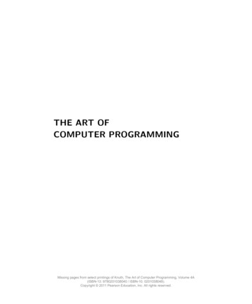
3Drawing a Line SegmentSince a line is infinite in its nature, we have to restrict ourselves to drawing line segments, which willa be reasonable representation of infinite line when going from one side of a screen to another. Thesimplest way to represent a line segment is to have the coordinates of its two end points. One wayof drawing a line segment will be simply starting with one end point and on the way of approachingthe other, turning on pixels.This approach resembles our experience of drawing a line segment on paper, but it poses twoquestions. First, on what criterion should we select a pixel? And second, if the criterion is set, howdo we efficiently select the required pixels? For the first question, let us define X as the pixel onrow r and column c, and the lines y r and x c running through X and intersecting at its center.We also denote L as the line segment with end points (x1 , y1 ) and (x2 , y2 ) where x1 x2 . We thenwill have a criterion when m 1/2 (m is the slope) as follows:Pixel X will be turned on if y1 r y2 , x1 c x2 and if the intersecting point ofx c and L is within the boundaries of X. We shall not be concerned with when the linecrosses x c at one of the boundaries of pixel X, because choosing either pixel adjacentto this boundary has no effect on our line representation.Notice that we are using the typical mathematical coordinate system with origin at the lower leftcorner despite most device manufacturers putting the origin at the upper left corner of a screen. Alsowe are going to use indices starting from 0 instead of 1. This is the typical approach in computerprogramming.This is for the case m 1/2. For future reference, we call it the gentle case. For the steepercase when m 1/2, we simply re-label the x-axis as the y-axis and y-axis as the x-axis. Whenlabels are interchanged, those two cases are basically the same. They both have the absolute valueof slope smaller than 1/2.But why do we bother to divide into two cases? We will see in a moment that this division intocases dramatically simplifies our problem of selecting pixels. When looking at Figure 1, we see thatpixel at (1, 1) is selected and turned as well as the pixel at (2, 2). The pixel at (0, 0) is not selectedeven though the line segment starts within its boundaries. The pixel at (2, 1) is not selected eithereven though there is a portion of the line segment running through it.4The First Algorithm: DDAThe first algorithm we are going to introduce is DDA. It stands for Digital Differential Analyzer.Before we start to see how the algorithm works, let’s first answer why we need to divide linedrawing into two cases and restrict ourselves only to the gentle case. Referring to Figure 1 andonly considering positive slope, notice that when the line segment starts from the pixel at (0, 0), itfaces two choices. If it is gentle enough, it will enter the pixel at (1, 0) and crosses x 1 beforeleaving it. Otherwise, it will go into pixel (1, 1) and cross its line x 1 before leaving it. However,it will never be able to reach the pixel (1, 2), because its slope is no larger than 1/2. Therefore weonly need to choose one out of the two possible pixels. Furthermore, we already know where the twopixels are located. If the pixel where the line segment starts is at row y0 and column x0 , the twopixels we need to choose from will both be in the next column x0 1. One of them will be in row x0 ,same as the original pixel. The other will be in row x0 1, only one level above the original pixel.Then our algorithm can be described as starting with one pixel, and scanning each column of pixelsfrom left to right. Every time when we are entering the next column, we either choose the pixel inthe same row as the pixel in the previous column, or we choose the pixel in the row one level abovethe pixel in the previous column. When the slope is negative, we still only have two pixels to choosefrom. If the pixel we start from is at (x0 y0 ), then the pixels we choose from are (x0 1, y0 ) and(x0 1, y0 1). For future explanations, we are going to use the grid in Figure 2 as representationof a screen. Notice the origin in the grid is the lower left corner of a rectangular screen. The pixelsbelow x-axis and the pixels to the left of y-axis are not shown on screen. For simplicity, the upperand right boundaries of the screen are not shown.2
y 2y 1y 0x 0x 1x 2Figure 1: Criterion on how to select a pixelyxFigure 2: A Screen of Pixels3
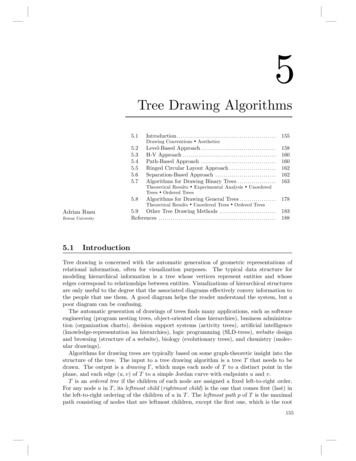
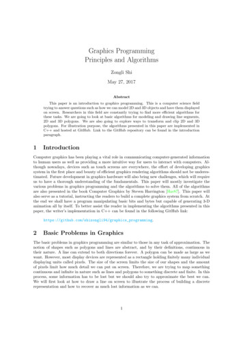
yP0B0xFigure 3: An Example of DDA AlgorithmyP1B1xFigure 4: The state of the program right after coloring a pixel in the second columnTo understand an algorithm, it is always helpful to have a sense of the idea behind it. ForDDA, when we are scanning the columns one by one, the movement from one column to another isessentially the same as adding 1 each time to the x-coordinate. Since a straight line has a constantrate of change, we can exploit this property by adding m, the value of slope, to the y-coordinateeach time we move to a new column. This is the idea behind DDA. To describe the implementationdetails, we define a crossing point to be the point where the line segment of interest crosses thecenter line of a column. We obtain the coordinates of first crossing point P0 as (x0 , y0 ) and distanceh between P0 and B0 , which is the central point of the row boundary right below P0 . We use h todetermine if we want to color subsequent pixels. When we move to the column x0 1, we add mto h. If h 1, we color the pixel (x0 1, y0 ). If h 1, we color the pixel (x0 1, y0 1) and wesubtract 1 from h. However, we can not use h to determine the first pixel we want to color becausethere is not a pixel in the previous color we can refer to. At column x0 , we simply color the pixel inrow ceil(y0 ). This seemingly arbitrary choice satisfies our criterion of coloring pixels. To illustratethis process, Let us have a line segment from (1.2, 2.1) to (8.7, 4.8). This line segment has a slopem 0.36 and is shown in Figure 3.Referring to Figure 3, the initial value of h is then around 0.208, which is the distance from B0to P0 . The first pixel in the second column and the third row will be colored as in Figure 4Referring to Figure 4, we find the new value of h to be 0.568 by adding m to the old h. Since4
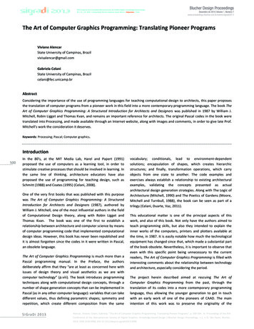
yP3B30xFigure 5: The state of the program right after coloring a pixel in the fourth columnyxFigure 6: The state of the program right after coloring a pixel in the fifth column0.568 1, we color the pixel in the same row in the third column. The procedure is repeated forthe fourth column as well, since the h for the third column is 0.928 1, we still color the pixel inthe same row. The result of coloring these two pixels is shown in Figure 5.Now when the line moves into the fifth column, the value of h becomes 0.928 0.36 1.288 whichis larger than 1. Therefore the pixel in the fourth row, which is one row above the previous coloredpixels, is colored. After coloring, we subtract 1 from h, since h is now measuring the distance fromP3 to B30 which is not the point on the closest boundary. To satisfy our definition of h, we subtract1 to prepare determining which pixel to color in the sixth column. The result of finishing this stepis shown in Figure 6What remains is simply repeating the steps we have done until we reach the last column wherewe need to color a pixel.5Bresenham’s algorithmAlthough the DDA algorithm is simple, it is not as efficient as it could be. One of the things thatslows it down is that DDA relies on floating point operations. If we can find a similar algorithmwhich only uses integer operations, then the new algorithm is going to be significantly faster thanDDA. Since drawing line segments is a common task in graphics programming, finding such an5
BAFigure 7: A line segment with integer coordinates at endpointsalgorithm will significantly improve the overall efficiency of the system. In the DDA algorithm, westore the value of h in memory to determine which pixel to color in the next column. The value of hserves as a criterion in determining rows, but in fact we do not really need to know the exact valueof h. At the end of computation in each column, the only thing we need to know is the Booleanvalue whether or not we need to color the pixel in the same row. If TRUE, we color pixel in thesame row. If FALSE, we color the pixel only one row above. Namely, we only need to know one ofthe two integers 0 or 1. Suppose we already colored the pixel in column x and row y, and we knowwhich pixel to color in column x 1. If there is a way we can determine which pixel to color incolumn x 2 based on the decision we made in column x 1, then the process of coloring pixels canbe improved by not having to adhere to a floating point value h. This is exactly where Bresenham’salgorithm excels.We will need a new criterion P instead of the old h and P has to be an integer otherwise thereis no improvement by using integer operations.We also need the line segment of interest to be specified with integer coordinates. If not, wesimply round the coordinates to make them integers.Now suppose we have a line segment specified by end points A and B with coordinates (m, n)and (m0 , n0 ) respectively where m, n, m0 and n0 are integers. Referring to Figure 7, we see the linesegment of interest. Since both end points have integer coordinates, they are located at the center ofa pixel. It is simple to draw the find the pixels occupied by A and B and color them. Now supposewe have drawn a pixel in column xk and row yk . We need to find out which of the two pixels tocolor in the next column xk 1. Since the pixels are adjacent vertically, it is natural to use distanceas a way of determination. This is depicted in Figure 8Denote the upper distance to be du and the lower distance to be dl . The three dots in Figure 8refer to the center of the pixel (yk 1, xk 1), the intersecting point of the line of interest and theline x xk 1, the center of the pixel (yk , xk 1) respectively from top to bottom. If the line ofinterest has an equation y mx b, then we can find the coordinates of point (xk 1, y):y m(xk 1) bThen we can find the value of the two distances:dl y yk m(xk 1) b ykdu yk 1 y yk 1 m(xk 1) b6
Figure 8: Use distances to determine which pixel to color in column xk 1[Tutb].To use the distances as a criterion, we only need the value d, which is the difference of them, todetermine which pixel to color:d dl du 2m(xk 1) 2b 2yk 1We multiply both sides with dx, which is equal to m0 m, or the difference between the x-coordinatesof the two end points:(dx)d 2(dy)(xk 1) 2(dx)b 2(dx)yk (dx) 2(dy)xk 2(dx)yk 2(dy) 2(dx)b (dx)The expression on the left side of the equation above will be the criterion we use as we are movingfrom column xk to column xk 1. This criterion will be used to determine which pixel to drawin column xk 1 and we already know which pixel has been drawn in column xk . Let’s denotepk (dx)d. If pk 0, we draw the lower pixel. Otherwise, we draw the upper one. Noticethat 2(dy) 2(dx)b (dx) will never change no matter in which column we are. Therefore letC 2(dy) 2(dx)b (dx), we have:pk 2(dy)xk 2(dx)yk CNow suppose we already determine which pixel to draw in column xk 1 using pk . As we are movingto column xk 2, we will need the value of pk 1 . Using the same process we have used to derive pk ,we derive pk 1 :pk 1 2(dy)xk 1 2(dx)yk 1 Cwhere (xk 1 , yk 1 ) is the pixel we colored using pk . Let’s subtract pk from pk 1 to get rid of theconstant term C:pk 1 pk 2(dy)(xk 1 xk ) 2(dx)(yk 1 yk )where we know xk 1 xk 1 since we are simply moving from one column to the next, therefore:pk 1 pk 2(dy) 2(dx)(yk 1 yk )Observe that the value of (yk 1 yk ) is either 0 or 1, because yk 1 is the row which we color incolumn xk 1 using pk . That is if pk 0, we have colored the pixel in the row yk . If pk 0, wehave colored the pixel in the row yk 1. Therefore, if pk 0, then:pk 1 pk 2(dy)7
Figure 9: Lines that look ragged and discontinuous due to information lossOtherwise, then:Pk 1 pk 2(dy) 2(dx)This implies that, given the truth value about whether pk is larger than 0, we can determine whichpixel to color in column xk 1, and at the same time we can determine pk 1 . In the processof determining pixels and finding criterion for the next column, only integer operations are usedbecause the end points have to have integer coordinates and the pi ’s we used are always integers ifthe first pi is an integer. The only thing left undone is to find the value of the first pi . This is thevalue of the criterion for coloring the second column covered by the line of interest. We have alreadycolored the pixel in the first column by directly using the coordinates of the starting point. Observethat if dy/dx 1/2, then we color the upper pixel. Otherwise we color the lower pixel. This if-thenstatement can be re-written using only integer operations as follows:p0 2(dy) (dx)where if p0 0, we color the the upper pixel. Otherwise we color the lower pixel. Therefore thechecking procedure for p0 is the same as other pi ’s.6Anti-aliasingSo far, we are capable of drawing a line on screen. However, we have not addressed the fact thatsome non-trivial information has been lost in the process of line generation. For example, lookingat the Figure 9, we see that the line we draw looks ragged and discontinuous. Figure 10 enlargesportion of Figure 9 to show the effect.The fact that some information is lost in the process of mapping something continuous in natureto a discrete space is called aliasing. This effect occurs when using digital medium to record musicand using digital camera to take photos. In most cases the effect will not be noticeable since moderntechniques use very short time interval to record sound and a large amount of pixels to encodeimages. However, in the case of line drawing, the problem of aliasing stands out and we have to dosomething to compensate for the lost information. The process of doing this is called anti-aliasing.8
Figure 10: Enlarged portion of Figure 9. Notice that the line is ragged and discontinuous.One way of reducing the raggedness of the line segment we draw is to color pixels in differentgrey scales. Notice in our original criterion of drawing line segments, for each column, only one pixelis drawn. However, the line may pass more than one pixel in a column. And even if the line passesonly one pixel in a column, it may not go though the center of a pixel. In Figure 1, even thoughthe line passes the pixel in row r and column c 1, we did not color it. It would be nice if we cancolor different pixels with different opacity value or gray scale according to how closely a pixel isrelated to the line of interest. One easy way of determining the opacity value is to find out howfar the center of a pixel is from the line segment and color the pixel with opacity value inverselyproportional to the distance. This algorithm is especially simple to implement in DDA because wealways keep a value of h in each column to measure the distance from one pixel to the line segment.A slight modification in DDA will enable us to make the line appear smoother and nicer to our eyes.Figure 11 is the line drawn with anti-aliasing. Figure 12 is an enlarged portion of 11. One thingwe should be careful about is that the opacity values in the pixels of one column should add up to1. If not, the line may appear thicker or thinner than it should be.More complicated algorithm can be used but more complication will not slow down our linegeneration algorithm so much. A simple scheme of calculating the grey scale values and storingthem in a table beforehand can guarantee the order of computation will only be increased by addinga constant term which is essentially ignorable. We will not go into more complicated line anti-aliasingalgorithm here. However, because of using integer operations exclusively, implementing anti-aliasingfor Bresenham’s algorithm is more involved than DDA. A common method of adding anti-aliasingto a line drawn using Bresenham’s algorithm is Xiaolin Wu’s algorithm. It is described in the paperAn Efficient Antialiasing Technique [Wu91] published in Computer Graphics.7Display FileUntil now, we have been able to draw straight lines on a screen. Later on we may wish to add morefunctions for drawing a circle, a polygon or even some 3D shapes. For the sake of good programmingpractice, we may want to encapsulate all the drawing functions into a single object. We will callthe object “drawer”. To specify the various instructions we may ask the drawer object to do, wewill need a display file. It will hold a list of instructions which will then be interpreted by anotherabstract class screen to draw on an actual physical screen. The purpose of a screen class is to hide9
Figure 11: Lines drawn with anti-aliasingFigure 12: Enlarged portion of Figure 1110
away the messy details for a specific type of screen. It also offers a common interface for differenttypes of screens, so our drawing commands in display file will be transportable across different kindsof hardware. The only assumption made about the three classes is that we restrict ourselves to drawon a rectangular screen and the pixels are represented as a grid.In order to make the display file more convenient to use, we maintain two pointers to indicate thecurrent drawing pen position. One point is for the x-coordinate. The other is for the y-coordinate.It is implemented by having three arrays. The first array will hold the integers called opcoderepresenting the types of commands. Currently we have two commands: a move command to movethe pen without leaving a trace with opcode 1 and a line drawing command with opcode 2 to movethe pen while drawing line on its way to the end points. The second array will hold the x-coordinateof the point to which we wish to draw a line or only move the pen. The third array holds they-coordinate of the same point. The indices are also shown on the left most column. An index i isused to identify the i-th command in our display file. A sample display file is shown below assumingthe initial pen position is (0, rpretationmove the pen to position (30, 25)draw a line segment between (30, 25) and (40, 40)draw a line segment between (40, 40) and (100, 20)draw a line segment between (100, 20) and (30, 25)move the pen to position (10, 0)Notice that we essentially draw a triangle with the command above and eventually the pen stops atposition (10, 0).Despite the fact that we have display file as a more concise specification about what we wantto draw on a screen, we should not try to write to the display file directly. Entering numbers iserror-prone and we have to stick with a particular implementation of display file. Instead of usingthree arrays, we may also implement display file as a single array containing a list of commandobjects representing individual commands. In other situations, we may also find linked list may bea better option than a non-expandable array. In other words, we need to encapsulate what we cando with display file and expose the functions as an abstract programming interface to the user. Wedefine four different functions for our API (abstract programming interface):draw line abs(x1 , y1 )move pen abs(x1 , y1 )draw line rel(dx, dy)move pen rel(dx, dy)Here, we use abs and rel as the abbreviations for absolute and relative. When we ask the displayfile to carry out an absolute command, we ask the drawer to draw or move from the current penposition to (x1 , y1 ). When we issue a relative command, we ask the drawer to draw or move fromcurrent pen position (x0 , y0 ) to the position (x0 dx, y0 dy). Although relative and absolutecommands are specified differently, they can implemented in the same way. Let current pen positionbe (x0 , y0 ), implementing relative commands is the same as implementing the absolute commandswith arguments (x0 dx, y0 dy). After converting every relative command to be absolute, we canenter all commands directly into display file regardless of being relative or absolute.In later sections, we will add more commands to enable us to draw more shapes on screen.8Polygon RepresentationOne of the straightforward applications of line drawing algorithms is to draw a polygon on screen aswe have done in the sample display file table. The only thing we need to do is to draw line segmentsone after another connected with each other. Our abstract representation of a pen in display file isespecially easy to use in this situation since we do not have to keep track of where one side of thepolygon ends to in order to draw another. However, before we start, we have think carefully abouthow we are going to represent a polygon abstractly. Some graphic systems use a set of trapezoidsto represent a polygon since any polygon can be broken into trapezoids. In those systems, drawing11
CBDAFigure 13: The shape drawn above has four five vertices and can be broken into two triangles butonly A, B, C and D are specified. The vertex at the center where line segments AB and CD crossis not specified and its coordinates remain unknowna polygon simply becomes drawing a set of trapezoids and only need to implement the procedurefor drawing a trapezoid. This implementation is doable but it forces the user to break a polygoninto trapezoids beforehand. It leaves the hard work and messy details to the user. Therefore itis error-prone to use and polygon drawing could be made easier and more flexible. An intuitiverepresentation of polygon to replace it would be a set of points representing vertices of the polygonof interest. It is then natural to implement drawing polygon as connecting the vertices in order. Theuser only has to specify a set of points in the correct order that he/she wants to use as vertices.Representing a polygon as a set of points is simple but there is a way that a user could misuseit. When representing a polygon as trapezoids, we can draw the polygon as convex or concave andwe know explicitly where the sides and vertices are. However, when drawing with a set of points,we may draw sides crossing each other. In this case, the crossing point of two sides should a vertexbut we have no information about it. This is shown in Figure 13. We may either rely on the userto check the vertices beforehand to make sure no lines are crossed but introducing difficulties tothe user is the problem we want to avoid at the first place. To allow more flexibility and keep thedrawing of a polygon simple to the user, we will allow lines to cross. Furthermore, in some cases itwould be even beneficial to allow line crossing. For example, look at Figure 14, we can draw a starwithout specify all of its 10 vertices even though it is a 10-gon.9Polygon FillingOnce we draw a polygon on screen, we may wish to fill it. Since we have written the procedure fordrawing line segments, scan line algorithm will be the most convenient to implement. Furthermore,most display devices nowadays have a scan line implemented in hardware one way or another.Therefore, scan line algorithm can be also very efficient. As the name of the algorithm implies, thereis a scan line which steps through each row of pixels on screen from top to bottom. When the scanline stops at a certain row, it first determines the points where the scan line intersects the polygonboundaries. For the coordinates of those points, it then decides which line segments to draw in orderto fill the polygon. Figure 15 illustrates this process.In Figure 15, we have a convex pentagon and one scan line shown. The scan line stop at y 3.The thick line segments between the intersecting points are the line segments we need to draw tofill the pentagon.Notice that our scan line does not have to step through every single row on a screen. For apolygon with several vertices, if we find the largest y-coordinate of those vertices, we essentiallyfind the y-coordinate the highest point. The same applies to the lowest point. Let’s denote the two12
DABCEFigure 14: Drawing a stare is made easier when we are allowed to draw lines crossing one another.To draw the shape shown above, we only need to specify 5 points as if it is a pentagon instead of 10.y 3Figure 15: Use scan line algorithm to fill a polygon. We first find the intersections of scan line andthe sides. Then we will draw horizontal line segments between each pair of intersection points usingthe existing line drawing function.13
PAFigure 16: Since the the horizontal AP has 3 intersection points with the sides of polygon, P is aninterior point.coordinates ymax and ymin . Then for our scan line y k where k is an integer determining whichrow our scan line is at, it only needs to move within the range where ymin k ymax .There is still one problem that remains. We do not know which line segments we have to chooseto draw. Obviously, the line segments within a polygon have the intersecting points as end points butwhich line segment is within a polygon? This is essentially the same to ask how we can determine ifa given point is inside a polygon. This question may be easy for humans to answer by only lookingat a picture but it is not so obvious for a computer to work it out. We are going to look at twodifferent algorithms for determining if a point is inside a polygon in the following two sections.9.1Even-odd rule/methodThe first algorithm we are going to consider is the even-odd method. This algorithm is intuitiveand easy to understand. Suppose we have a point P we are interested in determining if it is insidea polygon. First, let’s find a point A outside a polygon. An outside point is simple to find. We onlyneed the y-coordinate of A to be larger than ymax or smaller than ymin . Alternatively, we can alsohave the x-coordinate of A to be larger than xmax or smaller xmin (where xmax is the largest vertexx-coordinate). After selecting appropriate coordinates, we are sure A is outside the polygon.Now let’s connect AP . From Figure 16, we count the number of intersections of AP and rowboundaries. If AP happens to pass a vertex, we count it as 2 intersections because a vertex is sharedby two different boundaries. Suppose the total number of intersections is an integer n. If n is even,P is outside the polygon. Otherwise, P is inside.We can also think about even-odd method intuitively. Imagine the polygon of interest is a boxand we enter it from an outside point A. If we enter and stay, we cross the wall once. If we enterand leave, we are back to outside and we cross the wall twice. Any even number of crossing the wallwill make us outside. Any odd number of crossing will leave us inside. A special case is when wenever enter the box. The count of crossings is then 0 which is even. It is still true if we h
Principles and Algorithms Zongli Shi May 27, 2017 Abstract This paper is an introduction to graphics programming. This is a computer science eld trying to answer questions such as how we can model 2D and 3D objects and have them displayed on screen. Researchers in this eld are constantly trying to nd