Transcription
To appear, Proceedings of the IEEE Conference on Computer Vision and Pattern Recognition (CVPR), 2013.Deformable Spatial Pyramid Matching for Fast Dense CorrespondencesJaechul Kim1 Ce Liu2 Fei Sha3 Kristen Grauman1Univ. of Texas at Austin1 Microsoft Research New England2 Univ. of Southern crosoft.comAbstractfeisha@usc.eduedge on the images’ spatial layout, in principle we mustsearch every pixel to find the correct match.To address these challenges, existing methods havelargely focused on imposing geometric regularization onthe matching problem. Typically, this entails a smoothnessconstraint preferring that nearby pixels in one image getmatched to nearby locations in the second image; such constraints help resolve ambiguities that are common if matching with pixel appearance alone. If enforced in a naive way,however, they become overly costly to compute. Thus, researchers have explored various computationally efficientsolutions, including hierarchical optimization [15], randomized search [2], 1D approximations of 2D layout [11], spectral relaxations [13], and approximate graph matching [5].Despite the variety in the details of prior dense matchingmethods, we see that their underlying models are surprisingly similar: minimize the appearance matching cost ofindividual pixels while imposing geometric smoothness between paired pixels. That is, existing matching objectivescenter around pixels. While sufficient for instances (e.g.,MRF stereo matching [17]), the locality of pixels is problematic for generic image matching; pixels simply lack thediscriminating power to resolve matching ambiguity in theface of visual variations. Moreover, the computational costfor dense pixels remains a bottleneck for scalability.To address these limitations, we introduce a deformablespatial pyramid (DSP) model for fast dense matching.Rather than reason with pixels alone, the proposed modelregularizes match consistency at multiple spatial extents—ranging from an entire image, to coarse grid cells, to everysingle pixel. A key idea behind our approach is to strike abalance between robustness to image variations on the onehand, and accurate localization of pixel correspondenceson the other. We achieve this balance through a pyramidgraph: larger spatial nodes offer greater regularization whenappearance matches are ambiguous, while smaller spatialnodes help localize matches with fine detail. Furthermore,our model naturally leads to an efficient hierarchical optimization procedure.To validate our idea, we compare against state-of-theart methods on two datasets, reporting results for pixel la-We introduce a fast deformable spatial pyramid (DSP)matching algorithm for computing dense pixel correspondences. Dense matching methods typically enforce both appearance agreement between matched pixels as well as geometric smoothness between neighboring pixels. Whereasthe prevailing approaches operate at the pixel level, we propose a pyramid graph model that simultaneously regularizes match consistency at multiple spatial extents—rangingfrom an entire image, to coarse grid cells, to every single pixel. This novel regularization substantially improvespixel-level matching in the face of challenging image variations, while the “deformable” aspect of our model overcomes the strict rigidity of traditional spatial pyramids. Results on LabelMe and Caltech show our approach outperforms state-of-the-art methods (SIFT Flow [15] and PatchMatch [2]), both in terms of accuracy and run time.1. IntroductionMatching all the pixels between two images is a longstanding research problem in computer vision. Traditionaldense matching problems—such as stereo or optical flow—deal with the “instance matching” scenario, in which thetwo input images contain different viewpoints of the samescene or object. More recently, researchers have pushed theboundaries of dense matching to estimate correspondencesbetween images with different scenes or objects. This advance beyond instance matching leads to many interesting new applications, such as semantic image segmentation [15], image completion [2], image classification [11],and video depth estimation [10].There are two major challenges when matching genericimages: image variation and computational cost. Comparedto instances, different scenes and objects undergo muchmore severe variations in appearance, shape, and background clutter. These variations can easily confuse lowlevel matching functions. At the same time, the searchspace is much larger, since generic image matching permitsno clean geometric constraints. Without any prior knowl1
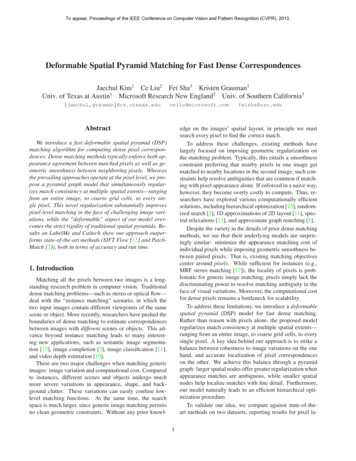
A imageAni Grid cells 2. Background and Related WorkWe review related work on dense matching, and explainhow prior objectives differ from ours.Traditional matching approaches aim to estimate veryaccurate pixel correspondences (e.g., sub-pixel error forstereo matching), given two images of the same scenewith slight viewpoint changes. For such accurate localization, most methods define the matching cost on pixels.In particular, the pixel-level Markov random field (MRF)model, combined with powerful optimization techniqueslike graph-cut or belief propagation, has become the defacto standard. It casts matching as a graph optimizationproblem, where pixels are nodes, and edges between neighboring nodes reflect the existence of spatial constraints between them [4]. The objective consists of a data term foreach pixel’s matching cost and a smoothness term for theneighbors’ locations.Unlike traditional instance matching, recent work attempts to densely match images containing different scenes.In this setting, the intra-class variation across images is often problematic (e.g., imagine computing dense matchesbetween a sedan and a convertible). Stronger geometric regularization is one way to overcome the matchingambiguity—for example, by enforcing geometric smoothness on all pairs of pixels, not just neighbors [3, 13] (seeFig. 1(c)). However, the increased number of pairwise connections makes them too costly for dense pixel-level correspondences, and more importantly, they lack the multi-scaleregularization we propose.The SIFT Flow algorithm pioneered the idea of densecorrespondences across different scenes [15]. For efficiency, it uses a multi-resolution image pyramid togetherwith a hierarchical optimization technique inspired by classic flow algorithms. At first glance it might look similar toour spatial pyramid, but in fact its objective is quite different. SIFT Flow relies on the conventional pixel-levelMRF model: each pixel defines a node, and graphs fromdifferent resolutions are treated independently. That is, nograph edges span between pyramid levels. Although pixelsfrom different resolution levels cover different spatial extents, they still span sub-image (local) regions even at thecoarsest resolution. In contrast, our model explicitly addresses both global (e.g., an entire image) and local (e.g.,a pixel) spatial extents, and nodes are linked between pyramid levels in the graph. Compare Figures 1(a) and (b). In bel transfer and semantic segmentation tasks. Comparedto today’s strongest and most widely used methods, SIFTFlow [15] and PatchMatch [2]—both of which rely on apixel-based model—our method achieves substantial gainsin matching accuracy. At the same time, it is noticeablyfaster, thanks to our coarse-to-fine optimization and otherimplementation choices. (c) Full pairwisemodel Pixels(a) DSP (Ours)(d) PatchMatch(b) SIFT FlowFigure 1. Graph representations of different matching models. Acircle denotes a graph node and its size represents its spatial extent.Edges denote geometric distortion terms. (a) Deformable spatialpyramid (proposed): uses spatial support at various extents. (b)Hierarchical pixel model [15]: the matching result from a lowerresolution image guides the matching in the next resolution. (c)Full pairwise model [3, 13]: every pair of nodes is linked for stronggeometric regularization (though limited to sparse nodes). (d)Pixel model with implicit smoothness [2]: geometric smoothnessis enforced in an indirect manner via a spatially-constrained correspondence search (dotted lines denote no explicit links). Asidefrom the proposed model (a), all graphs are defined on a pixel grid.addition, SIFT Flow defines the matching cost at each pixelnode by a single SIFT descriptor at a given (downsampled)resolution, which risks losing useful visual detail. In contrast, we define the matching cost of each node using multiple descriptors computed at the image’s original resolution,thus preserving richer visual information.The PatchMatch algorithm computes fast dense correspondences using a randomized search technique [2]. Forefficiency, it abandons the usual global optimization thatenforces explicit smoothness on neighboring pixels. Instead, it progressively searches for correspondences; a reliable match at one pixel subsequently guides the matchinglocations of its nearby pixels, thus implicitly enforcing geometric smoothness. See Figure 1(d).Despite the variations in graph connectivity, computation techniques, and/or problem domains, all of the aboveapproaches share a common basis: a flat, pixel-level objective. The appearance matching cost is defined at each pixel,and geometric smoothness is imposed between paired pixels. In contrast, the proposed deformable spatial pyramidmodel considers both matching costs and geometric regularization within multiple spatial extents. We show that thissubstantial structure change has dramatic impact on the accuracy and speed of dense matching.Rigid spatial pyramids are well-known in image classification, where histograms of visual words are often com-
pared using a series of successively coarser grid cells atfixed locations in the images [12, 20]. Aside from our focuson dense matching (vs. recognition), our work differs substantially from the familiar spatial pyramid, since we modelgeometric distortions between and across pyramid levels inthe matching objective. In that sense, our matching relatesto deformable part models in object detection [7] and sceneclassification [16]. Whereas all these models use a few tensof patches/parts and target object recognition, our modelhandles millions of pixels and targets dense pixel matching.The use of local and global spatial support for imagealignment has also been explored for mosaics [18] or layered stereo [1]. For such instance matching problems, however, it does not provide a clear win over pixel models inpractice. In contrast, we show it yields substantial gainswhen matching generic images of different scenes, and ourregular pyramid structure enables an efficient solution.3. ApproachWe first define our deformable spatial pyramid (DSP)graph for dense pixel matching (Sec. 3.1). Then, we definethe matching objective we will optimize on that pyramid(Sec. 3.2). Finally, we discuss technical issues, focusing onefficient computation (Sec. 3.3).3.1. Pyramid Graph ModelTo build our spatial pyramid, we start from the entireimage and divide it into four rectangular grid cells and keepdividing until we reach the predefined number of pyramidlevels (we use 3). This is a conventional spatial pyramid asseen in previous work. However, in addition to those threelevels, we further add one more layer, a pixel-level layer,such that the finest cells are one pixel in width.Then, we represent the pyramid with a graph. See Figures 1 (a) and 2. Each grid cell and pixel is a node, andedges link all neighboring nodes within the same level, aswell as parent-child nodes across adjacent levels. For thepixel level, however, we do not link neighboring pixels;each pixel is linked only to its parent cell. This saves usa lot of edge connections that would otherwise dominaterun-time during optimization.3.2. Matching ObjectiveNow, we define our matching objective for the proposedpyramid graph. We start with a basic formulation for matching images at a single fixed scale, and then extend it tomulti-scale matching.Fixed-Scale Matching Objective Let pi (xi , yi ) denote the location of node i in the pyramid graph, which isgiven by the node’s center coordinate. Let ti (ui , vi ) bethe translation of node i from the first to the second image.We want to find the optimal translations of each node in theIm1I 2Im2Grid cells (Fast and robust)Pixels (Accurate)Figure 2. Sketch of our DSP matching method. First row showsimage 1’s pyramid graph; second row shows the match solution onimage 2. Single-sided arrow in a node denotes its flow vector ti ;double-sided arrows between pyramid levels imply parent-childconnections between them (intra-level edges are also used but notdisplayed). We solve the matching problem at different sizes ofspatial nodes in two layers. Cells in the grid-layer (left three images) provide reliable (yet fast) initial correspondences that are robust to image variations due to their larger spatial support. Guidedby the grid-layer initial solution, we efficiently find accurate pixellevel correspondences (rightmost image). Best viewed in color.first image to match it to the second image, by minimizingthe energy function:XXE(t) Di (ti ) αVij (ti , tj ),(1)ii,j Nwhere Di is a data term, Vij is a smoothness term, α is aconstant weight, and N denotes pairs of nodes linked bygraph edges. Recall that edges span across pyramid levels,as well as within pyramid levels.Our data term Di measures the appearance matching costof node i at translation ti . It is defined as the average distance between local descriptors (e.g, SIFT) within node i inthe first image to those located within a region of the samescale in the second image after shifting by ti :Di (ti ) 1Xmin(kd1 (q) d2 (q ti )k1 , λ),z q(2)where q denotes pixel coordinates within a node i fromwhich local descriptors were extracted, z is the total number of descriptors, and d1 and d2 are descriptors extracted atthe locations q and q ti in the first and second image, respectively. For robustness to outliers, we use a truncated L1norm for descriptor distance with a threshold λ. Note thatz 1 at the pixel layer, where q contains a single point.The smoothness term Vij regularizes the solution by penalizing large discrepancies in the matching locations ofneighboring nodes: Vij min(kti tj k1 , γ). We againuse a truncated L1 norm with a threshold γ.How does our objective differ from the conventionalpixel-wise model? There are three main factors. First of all,
(a) Fixed-scale match(b) Multi-scale matchFigure 3. Comparing our fixed- and multi-scale matches. For visibility, we show matches only at a single level in the pyramid. In(a), the match for a node in the first image remains at the samefixed scale in the second image. In (b), the multi-scale objectiveallows the size of each node to optimally adjust when matched.graph nodes in our model are defined by cells of varyingspatial extents, whereas in prior models they are restrictedto pixels. This allows us to overcome appearance matchambiguities without committing to a single spatial scale.Second, our data term aggregates many local SIFT matcheswithin each node, as opposed to using a single match at eachindividual pixel. This greatly enhances robustness to imagevariations. Third, we explicitly link the nodes of differentspatial extents to impose smoothness, striking a balance between strong regularization by the larger nodes and accuratelocalization by the finer nodes.We minimize the main objective function (Eq. 1) usingloopy belief propagation to find the optimal correspondenceof each node (see Sec. 3.3 for details). Note that the resulting matching is asymmetric, mapping all of the nodes in thefirst image to some (possibly subset of) positions in the second image. Furthermore, while our method returns matchesfor all nodes in all levels of the pyramid, we are generallyinterested in the final dense matches at the pixel level. Theyare what we will use in the results.Multi-Scale Extension Thus far, we assume the matchingis done at a fixed scale: each grid cell is matched to anotherregion of the same size. Now, we extend our objective toallow nodes to be matched across different scales:E(t, s) XXXDi (ti , si ) αVij (ti , tj ) βWij (si , sj ).ii,j Ni,j N(3)Eq. 3 is a multi-scale extension of Eq. 1. We add a scalevariable si for each node and introduce a scale smoothnessterm Wij ksi sj k1 with an associated weight constantβ. The scale variable is allowed to take discrete values froma specified range of scale variations (to be defined below).The data term is also transformed into a multi-variate function defined as:1XDi (ti , si ) min(kd1 (q) d2 (si (q ti ))k1 , λ),z q(4)where we see the corresponding location of descriptor d2for a descriptor d1 is now determined by a translation tifollowed by a scaling si .Note that we allow each node to take its own optimalscale, rather than determine the best global scale betweentwo images. This is beneficial when an image includes bothforeground and background objects of different scales, orwhen individual objects have different sizes. See Figure 3.Dense correspondence for generic image matching is often treated at a fixed scale, though there are some multiscale implementations in related work. PatchMatch hasa multi-scale extension that expands the correspondencesearch range according to the scale of the previously foundmatch [2]. As in the fixed-scale case, our method has the advantage of modeling geometric distortion and match consistency across multiple spatial extents. While we handle scaleadaptation through the matching objective, one can alternatively consider representing each pixel with a set of SIFTs atmultiple scales [9]; that feature could potentially be pluggedinto any matching method, including ours, though its extraction time is far higher than typical fixed-scale features.Our multi-scale matching is efficient and works even withfixed-scale features.3.3. Efficient ComputationFor dense matching, computation time is naturally a bigconcern for scalability. Here we explain how we maintainefficiency both through our problem design and some technical implementation details.There are two major components that take most of thetime: (1) computing descriptor distances at every possibletranslation and (2) optimization via belief propagation (BP).For the descriptor distances, the complexity is O(mlk),where m is the number of descriptors extracted in the firstimage, l is the number of possible translations, and k is thedescriptor dimension. For BP, we use a generalized distance transform technique, which reduces the cost of message passing between nodes from O(l2 ) to O(l) [8]. Evenso, BP’s overall run-time is O(nl), where n is the numberof nodes in the graph. Thus, the total cost of our method isO(mlk nl) time. Note that n, m, and l are all on the orderof the number of pixels (i.e., 105 106 ); if solving theproblem at once, it is far from efficient.Therefore, we use a hierarchical approach to improveefficiency. We initialize the solution by running BP fora graph built on all the nodes except the pixel-level ones(which we will call first-layer), and then refine it at the pixelnodes (which we will call second-layer). In Figure 2, thefirst three images on the left comprise the first layer, and thefourth depicts the second (pixel) layer.Compared to SIFT Flow’s hierarchical variant [15], oursruns an order of magnitude faster, as we will show in the results. The key reason is the two methods’ differing match-
ing objectives: ours is on a pyramid, theirs is a pixel model.Hierarchical SIFT Flow solves BP on the pixel grids in theimage pyramid; starting from a downsampled image, it progressively narrows down the possible solution space as itmoves to the finer images, reducing the number of possibletranslations l. However, n and m are still on the order of thenumber of pixels. In contrast, the number of nodes in ourfirst-layer BP is just tens. Moreover, we observe that sparsedescriptor sampling is enough for the first-layer BP: as longas a grid cell includes 100s of local descriptors within it,its average descriptor distance for the data term (Eq. 2) provides a reliable matching cost. Thus, we don’t need densedescriptors in the first-layer BP, substantially reducing m.In addition, our decision not to link edges between pixels(i.e., no loopy graph at the pixel layer) means the secondlayer solution can be computed very efficiently in a noniterative manner. Once we run the first-layer BP, the optimaltranslation ti at a pixel-level node i is simply determinedby: ti arg min(Di (t) αVij (t, tj )), where a node j ista parent grid cell of a pixel node i, and tj is a fixed valueobtained from the first-layer BP.Our multi-scale extension incurs additional cost due tothe scale smoothness and multi-variate data terms. The former affects message passing; the latter affects the descriptordistance computation. In a naive implementation, both linearly increase the cost in terms of the number of the scalesconsidered. For the data term, however, we can avoid repeating computation per scale. Once we obtain Di (ti , si 1.0) by computing the pairwise descriptor distance at si 1.0, it can be re-used for all other scales; the data termDi (ti , si ) at scale si maps to Di ((si 1)q siti , si 1.0)of the reference scale (see supplementary file for details).This significantly reduces computation time, in that SIFTdistances dominate the BP optimization since m is muchhigher than the number of nodes in the first-layer BP.ApproachLT-ACCIOULOC-ERR Time (s)DSP (Ours)0.7320.4820.1150.65SIFT Flow [15]0.6800.4500.16212.8PatchMatch [2]0.6460.3750.2381.03Table 1. Object matching on the Caltech-101. We outperform thestate-of-the-art methods in both matching accuracy and speed.ApproachLT-ACC Time (s)DSP (Ours)0.7060.360SIFT Flow [15]0.67211.52PatchMatch [2]0.6070.877Table 2. Scene matching on the LMO dataset. We outperform thecurrent methods in both accuracy and speed.20. This reduction saves about 1 second per image matchwithout losing matching accuracy.1 For multi-scale match,we use seven scales between 0.5 and 2.0—we choose thei 4search scale as an exponent of 2 3 , where i 1, ., 7.Evaluation metrics: To measure image matching quality, we use label transfer accuracy (LT-ACC) between pixelcorrespondences [14]. Given a test and an exemplar image,we transfer the annotated class labels of the exemplar pixelsto the test ones via pixel correspondences, and count howmany pixels in the test image are correctly labeled.For object matching in Caltech-101 dataset, we also usethe intersection over union (IOU) metric [6]. Compared toLT-ACC, this metric allows us to isolate the matching quality for the foreground object, separate from the irrelevantbackground pixels.We also evaluate the localization error (LOC-ERR) ofcorresponding pixel positions. Since there are no availableground-truth pixel matching positions between images, weobtain pixel locations using an object bounding box: pixellocations are given by the normalized coordinates with respect to the box’s position and size. For details, please seethe supplementary file.4. ResultsThe main goals of the experiments are (1) to evaluateraw matching quality (Sec. 4.1), (2) to validate our methodapplied to sematic segmentation (Sec. 4.2), and (3) to verifythe impact of our multi-scale extension (Sec. 4.3).We compare our deformable spatial pyramid (DSP) approach to state-of-the-art dense pixel matching methods,SIFT Flow [15] (SF) and PatchMatch [2] (PM), using theauthors’ publicly available code. We use two datasets: theCaltech-101 and LabelMe Outdoor (LMO) [14].Implementation details: We fix the parameters of ourmethod for all experiments: α 0.005 in Eq. 1, γ 0.25,and λ 500. For multi-scale, we set α 0.005 andβ 0.005 in Eq. 3. We extract SIFT descriptors of 16x16patch size at every pixel using VLFeat [19]. We apply PCAto the extracted SIFT descriptors, reducing the dimension to4.1. Raw Image Matching AccuracyIn this section, we evaluate raw pixel matching quality intwo different tasks: object matching and scene matching.Object matching under intra-class variations: For thisexperiment, we randomly pick 15 pairs of images for eachobject class in the Caltech-101 (total 1,515 pairs of images).Each image has ground-truth pixel labels for the foregroundobject. Table 1 shows the result. Our DSP outperformsSIFT Flow by 5 points in label transfer accuracy, yet isabout 25 times faster. We achieve a 9 point gain over PatchMatch, in about half the runtime. Our localization error andIOU scores are also better.1 We use the same PCA-SIFT for ours and PatchMatch. For SIFT Flow,however, we use the authors’ custom code to extract SIFT; we do so because we observed SIFT Flow loses accuracy when using PCA-SIFT.
Ours ImaagesOSFPMPMSFOuurs ImagessFigure 4. Example object matches per method. In each match example (rows 2-4), the left image shows the result of warping the secondimage to the first via pixel correspondences, and the right one shows the transferred pixel labels for the first image (white: fg, black:bg). We see that ours works robustly under image variations like background clutter (1st and 2nd examples), appearance change (4th and5th ones). Further, even when objects lack texture (3rd example), ours finds reliable correspondences, exploiting global object structure.However, the single-scale version of our method fails when objects undergo substantial scale variation (6th example). Best viewed in color.Figure 5. Example scene matches per method. Displayed as in Fig. 4, except here the scenes have multiple labels (not just fg/bg). Pixellabels are marked by colors, denoting one of the 33 classes in the LMO dataset. Best viewed in color.Figure 4 shows example matches by the different methods. We see that DSP works robustly under image variations like appearance change and background clutter. Onthe other hand, the two existing methods—both of whichrely on only local pixel-level appearance—get lost underthe substantial image variations. This shows our spatialpyramid graph successfully imposes geometric regularization from various spatial extents, overcoming the matchingambiguity that can arise if considering local pixels alone.We also can see some differences between the two existing models. PatchMatch abandons explicit geometricsmoothness for speed. However, this tends to hurt matchingquality—the matching positions of even nearby pixels arequite dithered, making the results noisy. On the other hand,SIFT Flow imposes stronger smoothness by MRF connections between nearby pixels, providing visually more pleasing results. In effect, DSP combines the strengths of theother two. Like PatchMatch, we remove neighbor links inthe pixel-level optimization for efficiency. However, we cando this without hurting accuracy since larger spatial nodesin our model enforce a proper smoothness on pixels.Scene matching: Whereas the object matching task isconcerned with foreground/background matches, in thescene matching task each pixel in an exemplar is annotatedwith one of multiple class labels. Here we use the LMOdataset, which annotates pixels as one of 33 class labels(e.g., river, car, grass, building). We randomly split the testand exemplar images in half (1,344 images each). For eachtest image, we first find the exemplar image that is its nearest neighbor in GIST space. Then, we match pixels betweenthe test image and the selected exemplar. When measuringlabel transfer accuracy, we only consider the matchable pixels that belong to the classes common to both images. Thissetting is similar to the one in [14].Table 2 shows the results.2 Again, our DSP outperformsthe current methods. Figure 5 compares some examplescene matches. We see that DSP better preserves the scenestructure; for example, the horizons (1st, 3rd, and 4th examples) and skylines (2nd and 5th) are robustly estimated.2 The IOU and LOC-ACC metrics assume a figure-ground setting, andhence are not applicable here.
ApproachLT-ACC (GT) LT-ACC (GIST) LT-ACC (SVM)DSP (Ours)0.8680.7450.761SIFT Flow [15]0.8340.7590.753PatchMatch [2]0.7610.7040.701Table 4. Semantic segmentation results on the LMO dataset.PMMSFOursApproachLT-ACCIOUDSP (Ours)0.8680.694SIFT Flow [15]0.8200.641PatchMatch [2]0.8160.604Table 3. Figure-ground segmentation results in Caltech-101.Figure 6. Example figure-ground segmentations on Caltech-101.4.2. Semantic Segmentation by Matching PixelsNext, we apply our method to a semantic segmentationtask, following the protocol in [14]. To explain briefly, wematch a test image to multiple exemplar images, where pixels in the exemplars are annotated by ground-truth class labels. Then, the best matching scores (SIFT descriptor distances) between each test pixel and its corresponding exemplar pixels define the class label likelihood of the test pixel.Using this label likelihood, we use a standard MRF to assign a class label to each pixel. See [14] for details. Building on this common framework, we test how the differentmatching methods influence segmentation quality.Category-specific figure-ground segmentation: First,we perform binary figure-ground segmentation on Caltech.We randomly select 15/15 test/exemplar images from eachclass. We match a test image to exemplars from thesame class, and perform figure-ground segmentation withan MRF as described above. Table 3 shows the result. OurDSP outperforms the current methods substantially. Figure 6 shows example segmentation results. We see thatour method successfully delineates foreground objects fromconfusing backgrounds.Multi-class pixel labeling: Next, we perform semanticsegmentation on the LMO dataset. For each test image, wefirst retrieve an initial exemplar “shortlist”, following [14].The test image is matched against only the shortlist exemplars to estimate the class likelihoods.3 We test three different ways to define the shortlist: (1)
gle pixel. This novel regularization substantially improves pixel-level matching in the face of challenging image vari-ations, while the “deformable” aspect of our model over-comes the strict rigidity of traditional spatial pyramids. Re-sults on LabelMe and Caltech show our approach outper-forms state-of