WIXLIB

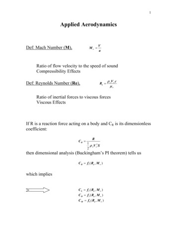
1Applied AerodynamicsDef: Mach Number (M),M VaRatio of flow velocity to the speed of soundCompressibility EffectsDef: Reynolds Number (Re),Re ρ V cµ Ratio of inertial forces to viscous forcesViscous EffectsIf R is a reaction force acting on a body and CR is its dimensionlesscoefficient:CR R1ρ V 2 S2then dimensional analysis (Buckingham’s PI theorem) tells usC R f1 ( Re , M )which impliesC L f 2 ( Re , M )C D f3 ( Re , M )C M f 4 ( Re , M )

2Your Fluid Mechanics Courses:Basic Fluid Mechanics Application of F ma to fluids Imcompressible Flows Mostly Inviscid (some pipe flow if you were lucky)Fundamental Aerodynamics Incompressible Flow Theory (no compressibility, noviscousity) Sources, sinks and vortices Panel Methods (2D only)Gas Dynamics Mach Number effects (mostly shock/expansion theory,supersonic flows) Possible corrections for high subsonic flowApplied Aerodynamics 3D Bodies Viscous Flows Compressibility Effects Aerodynamic Design IssuesInviscid 3D Wing TheoryViscous Airfoil Codes – Xfoil from MIT

3Class Plan: Review 2D Airfoil Theory (Chapters 3&4 of Anderson) Introduce 3D Wing Theory (Chapters 5&6) Navier-Stokes and Boundary Layer Equations XFOIL Applied Aerodynamics Design Concepts (along the way)

4Review of Airfoil Theory and 2D AerodynamicsElemental SolutionsFlows about 2D airfoils are built from four elemental solutions:uniform flow, source/sink, doublet and vortex. These elementalsolutions are solutions to the governing equations ofincompressible flow, Laplace’s equation. φ 0 ϕ 022(3.1)which relies on the flow being irrotationalr V 0(3.2)Equations (3.1) are solved forN - the velocity potentialR - the stream functionThe velocity potential is such thatrV φ ,i.e., u φ φ,v y x(3.3)whereas the stream function is always orthogonal (perpendicular)to the velocity potential,u ϕ ϕ,v y x(3.4)

5Convenient Coordinate SystemsCartesian: φ φ ( x , y, z ) φ φ φ φ 0 x y z222222(3.5)2Cylindrical: φ φ ( r ,θ , z )1 φ 1 φ φ 0 φ r zr r r r θ222222(3.6)Spherical: φ φ ( r ,θ , Φ ) φ 21r sin θ2 φ rsinθ r r θ2 sin θ φ 1 φ 0 θ Φ sin θ Φ (3.7)Big Advantage: Laplace’s Equation is LINEAR Superposition is possible

6Boundary ConditionsSolution about a specific body requires that the body be astreamline, i.e., flow tangency condition.rV nˆ 0or φ 0 n ϕ 0 s(3.8)where n- surface normal, s – surface tangentAnother way to say it is that the surface has to be a streamline:dy v dx ubstreamline equation

7Uniform Flowφ C1 x C 2ϕ C1 y C 3(3.9) ϕ φ C1 V y x φ ϕv 0 y xu In cylindrical coordinatesφ V r cosθϕ V r sin θ(3.10)

8Source/SinkcVr ,rVθ 0Λ Source Strength(3.11)v& 2πrVrlWhere v& is the volume flow rate (sometimes called Q)Vr SoΛln r2π φΛ Vr r 2πr1 φVθ 0r θφ Λ2πr(3.12)v& m&ρ(3.13)Λθ2π1 ϕΛVr r θ 2πr ϕ 0Vθ rϕ Def: Circulatiorn ':rΓ ( V ) ds V dsCif S is an area that includes the source, Γsource / sin k 0(3.14)(3.15)

9Superposition of Source and Uniform Flowϕ V r sin θ Λθ2π1 ϕΛ V cosθ 2πrr θ ϕVθ V sin θ rVr Stagnation Point – Set Λ, π 2πV (3.16)Vr Vθ 0(3.17)The stagnation point can now be used to define the bodystreamline, i.e., insert the stagnation point coordinates into thestream function equation to get its constant value. That newequation defines the body streamline.

10Superposition of Source, Sink and Uniform Flowϕ V r sin θ ΛΛθ1 θ 22π2π(3.18)Doublet FlowThe source and sink of the last section were separated by a distancel and they had identical strengths. If one imagines that their streamfunction is variable and their distance can be altered a newcondition would result if they are moved together while holdingconstant the product l7. In the limit, as l 0 a doublet is formed.φ K cosθ2π rϕ K sin θ2π r(3.19)where K l7. Streamlines are found by choosing R constant sothat we getr Ksin θ d sin θ2πc(3.20)

11Doublet Uniform FlowWhen a doublet is superposed together with a uniform flow we getthe flow over a circular cylinder.ϕ V r sin θ 2or if we let R KK sin θ2π r(3.21)2πV R2 ϕ V r sin θ 1 2 r (3.22)Velocities become:1 ϕ 1 R2 Vr V r cosθ 1 2 r θ rr R2 Vr 1 2 V cosθr 2R2 R2 ϕVθ V r sin θ 3 1 2 V sin θ rrr R2 Vθ 1 2 V sin θr (3.23-3.24)

12Stagnation Points are again found by setting the velocities to zero. R2 1 2 V cosθ 0r R2 1 2 V sin θ 0r (3.25)Which gives (R,0) and (R,B). The stagnation streamline thenbecomes R2 ϕ V r sin θ 1 2 0, i.e., r R, a circler (3.26)

13Pressure CoefficientFrom the Bernoulli Equation we get: V C p 1 V 2(3.27)Which becomes on the cylinderC p 1 4 sin 2 θ(3.28)From this we see that the axial and normal force coefficientsbecome:1cC n (C p , l C p , u )dxc01 TEC a (C p , f C p ,b )dyc LE(3.29)Both turn out to be zero since the pressure coefficient issymmetric. , i.e., D’Alembert’s paradox!

14Vortex Flowφ Γθ2πϕ Γln r2π(3.30)Γ1 φ r θ2πr φ 0Vθ rVθ rCirculation Γ V ds Vθ 2πr(3.31)C(r)But we also know that Γ V ds(3.32)How does this square if the flow is everywhere irrotational?Answer, it doesn’t, the flow is irrotational everywhere except at thecenter of the vortex. The angular velocity becomes infinite at thatsingularity.

15Doublet Uniform Flow Vortexr R2 Γϕ (V r sin θ ) 1 2 lnr 2π R 1 ϕ R 2 Vr 1 2 V cosθr θ r Vθ R Γ ϕ 1 2 V sin θ r 2πr r 2(3.33)(3.34)This time the stagnation points depend upon '.Γ 4πV RΓ 4πV RΓ 4πV R Γ R, sin 1 4πV R R, 3π22 Γ Γ2 3π R , 2πV 4π2 V ()

162 θ2sinΓΓ2C p 1 4 sin θ RVRVππ2 Γ(3.35)Cl RV Cd 0L′ q SC l ρ V ΓLift is directly proportionalto circulation

17Panel MethodsThe primary technique for low speed analysis (incompressibleflow) is the panel method. We will discuss two, the source panelmethod and the vortex panel method.Source Panel MethodTo begin consider what would happen if you stretched a pointsource/sink out over some curve in spaceDefined by the equationdφ λdsln r2π(3.36)where λ λ (s ) , s being the direction along the “source sheet.” Todetermine the potential at some point P(x,y) induced by the sourcesheet, one integrates Eq. 3.36 along the sheet.λdsln rπ2abφ ( x , y) (3.37)

18When combined with a uniform flow this yields the flow over anarbitrary body if λ λ (s ) is prescribed in such a way that thedesired body shape becomes a streamline.In general, it is difficult to find an analytical expression forλ λ (s) , so it is approximated either by a series of constantsource “panels” or by linearly varying source “panels.”The equation for the potential induced by the jth panel is thenλj φ j ln rij ds j2π j(3.38)Which gives the contribution to N at point P from panel j. Thepotential for the entire flow field then comes by summing thecontributions from all the panels. At the center of each panel is acontrol point at which the basic equation for the surface normalvelocity can be found from

19λi n λ j [φ ( xi , yi )] (ln rij )ds jVni ni2 j 1 2π j ni(3.39)j iThis is the normal velocity contribution at the control point fromonly the source sheet. However, what we want is the body to be astreamline, so we must have:V n Vni 0(3.40)This leads to the equation that can be solved for the λ j unknownsλi2λjI ij V cos β i 0j 1 2πn (3.41)j iwhere I is the integral in Eq. 3.39.The surface velocity on the body at the control point can then befound fromn λ Vsi [φ ( x i , yi )] j (ln rij )ds j sj 1 2π j s(3.42)once the λ j are found. Lastly, the integral can be evaluated as onpage 256 of the Anderson text and C p found from the Bernoulliequation.Unfortunately, since we are dealing only with sources and sinksthe lift and drag are both zero!!!

20Lifting AirfoilsThe problem of lift in general is bound up in the idea of circulationand hence requires vortices in the panel method, which we showedearlier to be the only elemental solution to exhibit circulation. Toaccommodate this we use an idea similar to the source sheet, thevortex sheetWhose potential is given by the equation1 bφ ( x, z ) θγds2π a(4.1)where γ γ (s ) .Circulation comes about from the vortices and is related directly tothe distribution of γ , via:bΓ γds(4.2)aFrom this point the entire thin airfoil theory can be developed(which should be reviewed) or one can follow the same approach

21used to develop the source panel method using the vortex sheetequation to produce a vortex panel method for arbitrary liftingbodies. However, one thing missing is the specification ofstagnation points.Which requires the Kutta Condition.Kutta ConditionThe basic idea is related to the fact that an infinite number ofstagnation point locations can exist on a lifting airfoil if only theearlier theory is applied, and because of that, virtually anycirculation (lift) is possible. However, Wilhelm Kutta observedthat the flow leaves a pointed trailing edge airfoil smoothly fromthe trailing edge, placing the stagnation point at the trailing edge.This is the so-called Kutta Condition and it provides the additionalinformation we need to determine the circulation and hence lift ofan arbitrary airfoil.

22Start-Up VortexAnother interesting, yet apparently contradictory, idea associatedwith airfoils comes about because of Kelvin’s Theorem, which sayscirculation does not change along a fixed fluid element. If it startsout zero around an airfoil at rest, it must remain zero along thatfluid element.For circulation to exist about the airfoil (and hence lift) it mustcoexist with an equal strength negative circulation shed at airfoilstart-up and convecting downstream bounded by the original fluidelement.

23Vortex Panel MethodSo just as in the source panel method, the vortex sheet can beapproximated by a series of discrete vortex panels of constant orvarying strength. Again the body must be a streamline and hencethe flow tangency condition can be applied at the control points.The resulting equation for vortex strength isγ j θ ijV cos β i ds j 0j 1 2π j nin(4.3)This produces a system of n unknowns and n equations. We think“good” but not so, because it still doesn’t incorporate the KuttaCondition. A way to do this is to make the trailing edge panelsvery small and enforceγ i γ i 1(4.4)as illustrated in the Figure below.Unfortunately, now the system is over determined. To obtain adeterminate system one must eliminate one of the panels from thelinear equation set. Then, once the system is solved, the lift can bedetermined directly from the known coefficients, i.e.,nL′ ρ V γ j s jj 1Next up Wing Theory!!!!(4.5)

streamline, so we must have: 0 n n i V V (3.40) This leads to the equation that can be solved for the λ j unknowns cos 0 2 1 2 i n j i j ij i j I V β π λ λ (3.41) where I is the integral in Eq. 3.39. The surface velocity on the body at the control p