Transcription
Seminar Corporate Governance:Topics on Data Analysis with STATAYuhao Zhuy.zhu@ese.eur.nl22 November 2017ContentsIIntroductory21 Why we are here and how we get there?22 What to learn today?2II3Databases3 Fantastic databases and how to find them34 WRDS4III4STATA5 Why STATA?56 STATA basics, commands, and do-files67 Basic commands with Demo98 Essential issues and common mistakes14IV19Tables9 Why tables are important?1910 A good table19VConclusion2211 Concluding remarks221
Part IIntroductory1Slide 2Why we are here and how we get there?Who am I? Yuhao (Hanan) Zhu. Final-year PhD Students at Erasmus School of Economics. Corporate Governance, Asset pricing, and Behavioral Finance.Slide 3Why this topic? Not knowing where to collect desired data. Lacking sufficient knowledge about STATA. Improperly resenting the results.Slide 4How to approach? Popular databases and what you can find from them. Basic knowledge of STATA commands, essential issues, and ability to read help documents. Design of the tables of results.Slide 5What to expect? Better data quality for your thesis. Correct results for your analysis. Clear way of showing your results.Slide 6Above allYou can improve your thesis grade by at least 1.0 if you do can reach these three criterion.2Slide 7What to learn today?Databases Popular databases. EDSC. WRDS.2
Slide 8STATA Layout. Idea behind STATA commands (functions). Link them to other computer languages. Basic commands for panel regressions. Essential issues and common mistakes. How to read STATA help document?Slide 9Tables How to get beautiful tables from STATA. How to get them into Excel? What items to show in your thesis? Title and captions.Slide 10Note Important sections and points are preceeded by an asterisk . There are two kinds of questions: questions and good questions. So feel free to ask. I will also ask questions during the lecture.Part IIDatabases3Slide 11Fantastic databases and how to find them Erasmus Data Service Center When you do not know which databases meet your need, go to the website of EDSC. https://www.eur.nl/ub/en/edsc/databases/financial databases/3
Slide 12EDSC - Financial databasesSlide 13Hand-collected data sets Sometimes, hand collected data sets are also important. Not all data you need for your thesis is available through data sets. You can collect them by hand or by spiders.4Slide 14 WRDSWRDS Wharton Research Data Services. https://wrds-web.wharton.upenn.edu/wrds/ You can get permission to WRDS through EDSC.Slide 15Databases Compustat: Fundamentals of the firm. Execucomp: Executive compensation. CRSP; Stock prices. Event Study: A nice tool to do event study.4
Part IIISTATA5Slide 16Why STATA?Too many choices Excel (VBA): We know them when we are very young. SPSS: The first statistical software you met in your bachelor. EViews R Matlab PythonSlide 17Advantages of STATA Ready-to-use packages and commands that are written and revised by previous researchers. Reusable codes and programs. Professional in handling panel data sets. In-design statistics.Slide 18Alternatives Excel (VBA and Python add-ins): Pre-process of the raw data sets. Some data setsare not clean enough for STATA. EViews: Professional in handling time-series analysis. R: Data visualization. Matlab: Simulations. Python: Spiders.Slide 19Job synergy Catch online data with Python. Pre-process and clean the data sets using Excel. Data visualization using R. Panel analysis using STATA.5
6STATA basics, commands, and do-filesSlide 20LayoutSlide 21Windows Input window: you give command to STATA. Output window: STATA gives you results. Review window: commands you typed before. You can reuse them by clicking. Variables window: List of variables within the data set. Property window: Property of a certain variable, e.g., name, label, and data type.Slide 22Give commands There are always two ways to give command: Click buttons in the menu bars or ribbons (like what you do in SPSS). Type your command and press ”Enter” (like what you do in CMD or Terminal).Slide 23Preferred way Typing command is preferred to clicking. Why? Clicking is annoying. Commands can be re-used later. We have ”do-file”.Slide 24Commands Commands are the most essential advantage of STATA. Clicking menu bars is first translated to commands, and then executed by STATA. Commands are well-defined functions! When you give commands, think that you are programming!6
Slide 25Idea behind commands Typed-in commands are conceptually equivalent to functions used in other computerlanguages. Y F unction (X1 , X2 , X3 , · · · θ). X1 , X2 , X3 and so on are the input arguments (independent variables). θ is the parameters (optional variables). Y is the output (dependent variable). F unction is well-defined sequential calculations and actions. Define once, and can bere-used many times.Slide 26Structure of the STATA commands command [arg1 arg2 .][if expression] [, options] Command name. main argument. optional arguments. sample constraints. options. ”Commands” are ”Functions” without parenthesis.Slide 27An example: OLS estimate What if we calculate the OLS estimate by hand? Independent variable(s): Matrix X. Dependent variable: Y. 1 OLS estimate b (X 0 X)X 0Y . This formular can be defined as a function: regressSlide 28An example: STATA We type the command: regress Y X STATA analyzes your command: The function is regress. The OLS estimate should be used. The first argument is Y. It is the dependent variable. The second argument is X. It is the independent variable. STATA conducts calculation in the background: b (X 0 X) b is printed in the output region.7 1X 0Y .
Slide 29An extended example: STATA We type the command: regress Y X if year 2000, vce(robust) The function is regress. The OLS estimate should be used. The first argument is Y. It is the dependent variable. The second argument is X. It is the independent variable. STATA sees if. So the sample is constrained to observations with year equal to 2000. STATA sees ,. So vce(robust) is option: using robust standard error.Slide 30 The most important things to learn about STATA commands The purpose of the command (function). The main arguments (variable) of the function. Which observations (sub-sample) are used? The options.Slide 31Example summarize age income if gender 1, detail The purpose of the function is to summarize the variables. The variables we want to summarize are age and income. Which observations are used: males. We want to show more detailed summary: , detailSlide 32What is do-file? A sequence of commands just like a program. Automatically run from the beginning to the end. Or run the selected parts. Easy to re-use the codes. Ready to show to others with comments. Loops.Slide 33Always use do-files Always use do-files when you use STATA. Ctrl D on PC, or Shift Cmd D on Mac to run selected commands.8
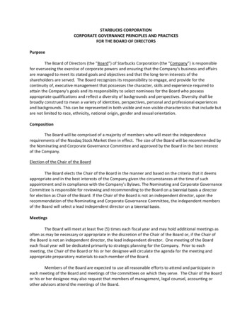
7Slide 34 Basic commands with DemoBasic functions We will go through basic commands (functions) for panel analysis by: The idea behind commands. The structure of a command. A real example.Slide 35Learning by doing Now we introduce the most basic commands in STATA. They are frequently utilizedwhen doing corporate finance studies. Get familiar with them for your thesis. Example: a German panel data set. Working paper: The real costs of CEO compensation: the effect of behindness aversionof employees. Purpose: Relationship between CEO compensation and workers’ pay.Slide 36Real example Data set 1: Firm-level information on 100 largest German firms (CEO compensationand performance) Data set 2: Branch-level (establishment-level) information (workers’ pay and laborstructure) Data set 3: Match book of the firm ID and the branch (establishment) ID.Slide 37Data structureEstablishmentCEOCEO compensation and personalinformation.FirmFirm-level characteristics, e.g.,performance, size, capital structure blishmentEstablishmentWorkers’ wages and establishment-levelcharacteristics, e.g., number of workers,proportion of different kinds of workersand etc.9
Slide 38Organize your folder Organize your folder for better readability. A parent folder, and several sub-folders. /orig: Contains original data sets. Do not change data sets in this folder. /data: Contains modified or intermediate data sets saved for further analysis. /prog: Do files. Other sub-folders if needed.Slide 39Create a do-file We need to create a do-file. Save it under ”analysis/prog/” Save the file in time.Slide 40Locate the path of the parent folder Locate your parent folder. For example, it is named ”analysis”. cd "C:\Data\.\guest lecture\analysis"Slide 41Open a data set We begin with open a data set. use "orig/firm level data.dta", clearSlide 42Generate variables generate ln market capital ln(market cap)gen return on asset ebitda / total assetSlide 43Summarize Summarize the variables. Missing values are not summarized. With option detail, you can obtain more detailed descriptions including quantiles. summarize ceo total market cap total salessum ceo total, detail // Show more details.Slide 44Correlation matrix You can create correlation matrix of many variables. correlate ceo total ceo cash board totalcorr market cap total sales employees10
Slide 45Sort Sort by variable name(s). sort market capsort market cap total salessort id iab // Sort firm id.Slide 46Merge data sets Step 1: Find the common key(s) Step 2: Identify the matching mode: 1-to-1, m-to-1, or m-to-m. Step 3: Decide the master and the using data sets.Slide 47Command joinby Syntex: joinby [varlist] using filename [, options] sort id iab // sort before joinbyjoinby id iab using "orig/match book.dta"Slide 48Command merge Syntex: merge m:m varlist using filename [, options] * Many-to-many matchingmerge m:m betnr year using "data.dta"* Keep only mathced observationskeep if merge 3* Drop the auto-created variabledrop mergeSlide 49Rename variables You maybe want to rename variables to make them easily recognized. rename id iab firm idrename betnr branch idSlide 50Handle duplicates Sometimes there are duplicates within sample. For example, for each branch and each year, there should be only one variable. But there are some times multiple values (mistakes during data collection, or justchange of id). duplicates drop branch id year, force11
Slide 51Generate dummy variables We need dummy variables for descriptive information. For example, we want to create a dummy indicating whether the union within the firmis ”igmetall”. * Generate a dummy with value 0.gen is igmetall 0* Change it to 1 under certain conditions.replace is igmetall 1 if union "igmetall"Slide 52Generate fixed effects dummies If you want to do regressions with fixed effects, you need to create dummies. STATA create N new dummy variables for N groups. tabulate year, generate(year fe )tabulate id iab, generate(firm fe )tabulate state branch, generate(state fe ) For example, year dummies: year fe 1, year fe 2, and so on.Slide 53Save modified data sets After modifications, we can save our data sets that are ready to be used for analysis. The option replace is important! save "data/panel data zhu.dta", replaceSlide 54Begin regressions Now we can use the modified data sets to do regressions. clear alluse data/panel data zhu.dta, clearSlide 55Declare data structure Before panel analysis, you need to declare the data structure. Time series, cross-sectional, or panel data set. For panel data set: xtset [group] [time]. For time series data set: tsset [time]. This enables time operators l.year, f.year, or l2.year. xtset branch id year12
Slide 56OLS Example 1: Normal OLS with 1 explanatory variable. regress ln worker wage ln ceo totalSlide 57OLS Example 2: Normal OLS with multiple explanatory variables. reg ln worker wage ln ceo total ///return on asset leverage ratioSlide 58OLS Example 3: OLS when year is after 2006. reg ln worker wage ln ceo total ///return on asset leverage ratio ///if year 2006Slide 59OLS Example 4: OLS when year is after 2006, using robust standard errors. reg ln worker wage ln ceo total ///return on asset leverage ratio ///if year 2006, vce(robust)Slide 60OLS Example 5: OLS when year is after 2006, using robust standard erros, with firm fixedeffects. reg ln worker wage ln ceo total ///return on asset leverage ratio ///firm fe * ///if year 2006, vce(robust)Slide 61OLS Example 6: OLS when year is after 2006, using robust standard erros, with multiplefixed effects. reg ln worker wage ln ceo total ///return on asset leverage ratio ///firm fe * year fe * state fe * ///if year 2006, vce(robust)13
Slide 62OLS Example 7: One-year lagged OLS when year is after 2006, using robust standard erros,with multiple fixed effects. reg ln worker wage l.ln ceo total ///return on asset leverage ratio ///firm fe * year fe * state fe * ///if year 2006, vce(robust)8Slide 63 Essential issues and common mistakesEssential issues Some issues are very essential when doing analysis or writing do-files with STATA. If you neglect these issues (or even ignore them), you may get error reports. Of course, your results are probably wrong! If your supervisor or co-reader detect this,then. Sometimes, remember these issues will save your a lot of time and energy. Time ismoney.Slide 64Write comments Comments start with *, //, or be blocked by /* and */. Sometimes you forget what you wrote yesterday. So use comments to remind yourself. If you want to show your do-file to others, comments may help.Slide 65Example: comments* This is a single-line comment.[commands]// This is also a single-line comment.[commands]/*This is a block of comments.*/Slide 66Line break Sometimes it is hard to write everything in a single line. Use [ ///] (one space and three slashes) to break lines for your commands.14
Slide 67merge or joinby Sometimes you need to think which merging command to choose. merge and joinby should generate the same results. However, under certain circumstances, one is superior to the other. joinby creates all pair-wise matching. Suppose that you think you are doing 1-to-1,m-to-1, or 1-to-m matching. However, there is duplicate observations in your sample.joinby will not report his error, but merge does. merge is not encouraged to do m-to-m matching! The matching is unstable! You getdifferent results every time you re-run this command.Slide 68Decision: merge or joinby merge for 1-to-1, m-to-1, or 1-to-m matching. joinby for m-to-m matching. Remember: I warned you.Slide 69Missing values Missing values should be treated carefully! Otherwise, you make mistakes.Slide 70Missing values: problem 1 If most of the observations for prop female are missing. You dropped missing values during data preparation. Compare the following codes: use data/panel data zhu.dta, clearregress ln worker wage ln ceo total use data/panel data zhu.dta, clearkeep if prop female .regress ln worker wage ln ceo total Your sample size will shrink! You are measuring only local treatment effect. So, do not drop missing variable if the variable is a trivial one!. STATA automaticallydrop them during regressions.Slide 71 Missing values: problem 2 I want to regress for branches where more than half of the workers are female. Comparethe following codes: use data/panel data zhu.dta, clearkeep if prop female ! .keep if prop female 0.5regress ln worker wage ln ceo total15
use data/panel data zhu.dta, clearregress ln worker wage ln ceo total ///if prop female 0.5 use data/panel data zhu.dta, clearregress ln worker wage ln ceo total ///if prop female 0.5 & prop female ! . Wrong sample during regression! Why?Slide 72 Missing values are treated as very large numbers Missing values . are treated as very large values in STATA. Compare the followingcodes: use data/panel data zhu.dta, clearkeep if prop female 1count prop female if prop female . use data/panel data zhu.dta, clearkeep if prop female 1count prop female if prop female . Do always treat missing values carefully!Slide 73Fixed effects What is fixed effects? How we add them into the regression? Fixed effects. i. or fe *Slide 74Do not use command xtreg Many students love to use the command xtreg. Do not use it! use "orig/firm level data.dta", clearxtset id iab yearxtreg ceo total employees, fereg ceo total employees i.id iab Drawback 1: xtreg does not report overal R-square and adjusted R-square. Notcomparable to OLS. Drawback 2: xtreg does not report coefficients for FE dummies. Drawback 3: It is hard to incorporate multiple fixed effects with xtreg. Drawback 4: t-statistics are more robust using FE dummies than using xtreg.16
Slide 75Fixed effect regressions: alternative methods Choice 1: create dummies and include them in the regression. firm fe * means all variables starting with firm fe . reg ln worker wage ln ceo total ///firm fe * year fe * state fe *Slide 76Fixed effect regressions: alternative methods Choice 2: use operator i. It only applies to numerical catagorical variables. reg ln worker wage ln ceo total ///i.firm id i.year i.state branch Following codes give error report: reg ln worker wage ln ceo total i.unionSlide 77Operations within groups Sometimes we need to do operations only within groups. For example: generate increase rate for each firm. Common mistake: inter-group increase rate. Always be careful when you are handling lagged data.Slide 78Row identifier Cells can be located by variable name and row identifier [ n]. Handling lags with row identifier. Remember to sort before handling data. sort id iab yeargen roa increase ///(roa[ n] - roa[ n-1]) / roa[ n-1] What is the problem left? Inter-group increase rate! Drop them!17
Slide 79Alternative ways Method 1: Use by command to identify groups. by id iab: gen roa increase ///(roa[ n] - roa[ n-1]) / roa[ n-1] Method 2: Use xtset command to specify the panel data set. Then use lagging operators. xtset id iab yeargen roa increase (roa - l.roa) / l.roaSlide 80by command by is equal to looping the command for each group. by id iab: sum roa We can do this also by looping. levelsof id iab, local(id)foreach i of local id {display "id iab ‘i’"sum roa if id iab ‘i’}Slide 81Third-party packages Some functions are programmed by third-parties. For example: IV regression, table output, winsorizing, and etc. Can be installed by commands: ssc install [package]. Be careful in selecting third-party packages, especially about historical versions.Slide 82Winsorizing Sometimes we need to winsorize the outliers. What is winsorizing? For the first time you use the package: ssc install winsor Now we conduct single-sided winsorizing to the observations whose value exceed 99%percentile. winsor prop female ///, generate(prop female winsor) p(0.01) highonlysum prop female, detailsum prop female winsor, de18
Slide 83Help with commands When you are not familiar with a new command, read the help documents. Type help [command]. Read syntax in the pop-out window. Click ”[R] command – purpose of the command” in the pop-out window. Read more detailed descriptions in ”STATA BASE REFERENCE MANUAL”Slide 84Learn to read documentations A typical STATA syntax goes as follows. regress depvar [indepvars] [if] [in] [weight] [, options] Also important: Description, Options, Stored results, and of course, Examples. Demo.Part IVTables9Slide 85Why tables are important?Tables An organized way of showing your results. A good table (figure) is better than 1000 words.Slide 86Above allWe do not read your sentences that carefully. We read your tables!10Slide 87 A good tableStructure A good title. Well-written descriptive words (caption). A nice table with necessary statistics.19
Slide 88Title Numbering: Table 1, Table 2, and so on. The purpose of your table. Not too long. Example: ”Summary statistics”. Example: ”CEO compensation and workers’ pay: Baseline regressions”.Slide 89Caption The caption should include all information about what you are testing, so that readersdo not need to refer to the main context. You need to specify: The purpose of your regressions (what relationship you want to test). The methods you are using (OLS, IV regression, Difference-in-difference, Probit model). The dependent variable and independent variables. Special settings. How standard errors are treated or clusterd? How t-statistics and significant levels are expressed.Slide 90Caption: an exampleThis table presents results for regressions with the annual wage of employees as the dependent variable. All independent variables are lagged by one year. See Table 1 for adetailed overview of variable definitions. In specification (3), we consider the observationsafter 2006 only. We use the White (1980) robust standard errors clustered at firm level.The t-statistics are reported below the estimates. ***, ** and * indicate that the value issignificantly different from zero at the 1%, 5% and 10% levels.Slide 91Table What information is necessary: Dependent variable and independent variables. Coefficients. t-statistics Significance level. R-square or adjusted R-square. Number of observations.20
Slide 92STATA table output The build-in table is not desirable. Only one regression per table. Hard to compare between models. Too long if fixed effects are included. We do not need them! Standard error, t-statistics, and p-value: Redundant. Confidence interval, F-statistics, Root MSE: we do not need them. Too long notes of collinearity.Slide 93t-statistics and p-value Reject the null hypothesis at the 95% level if t-statistics is located in the white region. To know about significant level, simply count stars.Slide 94We design our own table Use thrid-party package estout to generate concise and beautiful tables. Ready to be included in your thesis. No redundant output printed on your screen.Slide 95Command estout Install it for the first time. Use command quietly before regress Save statistics using estout store [name] Show the table with following commands. estout m *, ///cells(b(star fmt(%9.3f)) t(fmt(%9.2f))) ///style(fixed) title(Regression Results) ///stats(r2 a N, fmt(%9.3f %9.0f)) ///starlevels(* 0.10 ** 0.05 *** 0.01) ///drop(*industry fe* *year fe* *state fe*)21
Slide 96Export STATA table, a demo Copy as table. Modifications in Excel. Copy into Word / Powerpoint as pdf.Slide 97OutcomeDep. Var.ln(CEO total)model 1-0.001-0.27model 2-0.007-1.32model 10.00113224ln(workers' wage)model 4model 5-0.002-0.02-0.21-1.5model 6-0.023*-1.65ln(CEO total) (t-1)ROALeverage ratioMarket-to-book ratioln(total sales)After 2006Robust std errorFirm fixed effectsYear fixed effectsState fixed effectsConstantAdj. R squareObs.Slide 7***45.740.01213224Advantage of estout All necessary information is included. Comparable between different models. Ready to be used in your thesis.Part VConclusion11Slide 99Concluding remarksWhat we learnt Databases. STATA. Design your esYesYesYesYes10.106***43.850.01813224model 0.57YesYesYesYesYes10.340***22.380.0199631
Slide 100Questions Thank you for your attention. Please feel free to ask questions.23
Slide 34 Basic functions We will go through basic commands (functions) for panel analysis by: The idea behind commands. The structure of a command. A real example. Slide 35 Learning by doing Now we introduce the most basic commands in STATA. They are frequently utilized when doing corpora