Transcription
Neyeloff et al. BMC Research Notes 2012, HNICAL NOTEOpen AccessMeta-analyses and Forest plots using a microsoftexcel spreadsheet: step-by-step guide focusingon descriptive data analysisJeruza L Neyeloff1*, Sandra C Fuchs1,2 and Leila B Moreira1,2AbstractBackground: Meta-analyses are necessary to synthesize data obtained from primary research, and in manysituations reviews of observational studies are the only available alternative. General purpose statistical packagescan meta-analyze data, but usually require external macros or coding. Commercial specialist software is available,but may be expensive and focused in a particular type of primary data. Most available softwares have limitations indealing with descriptive data, and the graphical display of summary statistics such as incidence and prevalence isunsatisfactory. Analyses can be conducted using Microsoft Excel, but there was no previous guide available.Findings: We constructed a step-by-step guide to perform a meta-analysis in a Microsoft Excel spreadsheet, usingeither fixed-effect or random-effects models. We have also developed a second spreadsheet capable of producingcustomized forest plots.Conclusions: It is possible to conduct a meta-analysis using only Microsoft Excel. More important, to ourknowledge this is the first description of a method for producing a statistically adequate but graphically appealingforest plot summarizing descriptive data, using widely available software.BackgroundMeta-analyses and systematic reviews are necessary tosynthesize the ever-growing data obtained from primaryresearch. Performing a search on Pubmed limiting tothe type of article, the Mesh term “meta-analysis” willwield 4223 results in 2010 only. Although reviews ofinterventional studies, especially clinical trials, providethe best evidence, there are several situations in whichobservational studies are the only alternative. Meta-analyses of these studies are becoming more common, particularly after publication of the MOOSE statement [1].Some of the studies are not concerned with the assessment of relative risks or odds ratios, but are focused ona summary statistics of incidence or prevalence.General purpose statistical packages such as SPSS,Stata, SAS, and R can be used to perform meta-analyses,but it is not their primary function and hence they allrequire external macros or coding. These can be* Correspondence: jeruza med@yahoo.com.br1Post Graduate Program of Cardiology, Universidade Federal do Rio Grandedo Sul, Porto Alegre, BrazilFull list of author information is available at the end of the articledownloaded, but are not always easy for the researcherto understand or customize. Additionally, the first threeprograms do not have free access, with prices rangingfrom 250 to over 30,000 depending on version andcountry. R is a very resourceful open source package,but its use in health is still limited, due mostly to theneed of programming instead of a point-and-clickinterface.There are some software packages specifically developed to conduct meta-analyses. RevMan [2] is a freeware program from the Cochrane Collaboration thatrequires the researcher to fill all steps of a systematicreview. It only accepts effect sizes in traditional formats.Metawin [3] and Comprehensive Metanalysis (CMA) [4]are commercial software that have user friendly interfaces. The former only accepts three types of primarydata, while the latter has a purchase cost, but acceptsmore types of data. It can perform advanced analyses,but there are still limitations regarding graphic display,particularly of descriptive data, since CMA does notallow customization of the forest plot produced. Finally,there is also Meta-Analysis Made Easy (MIX) [5], an 2012 Neyeloff et al; licensee BioMed Central Ltd. This is an Open Access article distributed under the terms of the Creative CommonsAttribution License (http://creativecommons.org/licenses/by/2.0), which permits unrestricted use, distribution, and reproduction inany medium, provided the original work is properly cited.
Neyeloff et al. BMC Research Notes 2012, -on for Excel. It can be used for analysis of descriptive data selecting the input type to “continuous”, butthe free version does not allow for analysis of originaldata, only build in datasets. Some other options are nolonger available, as FAST*PRO [6], and others are stillcurrently under development, as Meta-Analyst [7].Another option would be to analyze data usingdirectly Microsoft Excel. Although it has a purchasecost, it is usually already installed in most computers,bundled with Microsoft Office package. Most researchers would be uncomfortable entering all the formulasthemselves, since they may seem complex at first. However, if the calculations are done in steps, statistics likeQ and I2 can be computed with basic arithmetic operations. Borestein et al [8] cites the impossibility of producing forest plots as an important limitation, but we havedeveloped a method to turn a scatter plot into a statistically correct forest plot, allowing the researcher to takeadvantage of all excel formatting tools. Our work isseparated into two spreadsheets, so researchers can useboth to conduct all calculations or simply the secondone if they have already analyzed the data in any othersoftware, but want an appealing graphical way of presenting it [Additional file 1].FindingsTechnical notesThe method described here was designed on a laptopwith Intel Core Duo 2.2 GHz processor, 4 GB RAM,running Windows Seven 64 bit and Microsoft OfficeExcel 2007. The spreadsheets were later tested on Excel2003, with no differences found in either the calculations or graphs.The outcome of meta-analyses is the effect summary.However, some reviews may only aim in combiningrates or prevalences; technically these cannot be called“effects”, since there is nothing “causing” it, and the correct term would be single group summary. We will referto both these estimates simply as “outcome” in order toavoid confusion, and maintain only the abbreviation ases to follow textbooks standard.Since we have established that the limitation of the existing software packages is handling descriptive data, we willbe using rates in our example so that the difference in thefinal forest plot is more overt. The data could be the prevalence of smoking in a country or the incidence of myocardial infarction in high risk patients. We chose to usetheoretical numbers so we could openly distribute thespreadsheets, test particular formulas and compare resultsobtained with other software. All formulas are presentedin traditional equations and also in excel format.Steps 1 and 2 always require adjustments according tostudy type and outcome. Columns in light grey inspreadsheet 1 are the ones to be adapted, while columnsPage 2 of 6in dark grey do not require any modification regardlessof study type (this includes all further steps of theguide). The necessary adjustments can be easily foundon methodological books [8-10].Cell B14 should be filled with the number of studiesbeing analyzed. There are annotations on the spreadsheet that pop up when the mouse pointer is uponselected cells, so the downloaded file can be used without constant consultation of the full article. The explanation for the formulas and detailing of steps are notpresent on the spreadsheet though. A recently publishedpaper by Schriger et al [11] reviewed over 300 systematic reviews and highlighted important aspects of producing forest plots, which were considered in developingthis approach.Steps in analyzing data and producing a forest plotSpreadsheet 1-analysis (Figure 1)1. Calculating the outcome (effect size, es)In our example we have the number of events and thenumber of subjects in columns B and C, so we can simneventsply compute the rate in column D asor D3 ntotalB3/C3 in Excel. It is the same from D3 to D12, andcopy and paste will automatically adjust the cell numbers. This copying and pasting should be done for steps1 through 6 and in step 9 B.1.2. Calculating Standard Error (SE)All SE can be derived from the formula (x̄ µ)2, but there are simplified derived equaSE ntions for different types of studies. Since we are using eseventsor SE , therates, we can use SE es*nnsame formula used in CMA. In excel this will be E3 D3/SQRT(D3*C3).3. Computing variance (Var)This formula is simple: Var SE 2 . In Excel, F3 E3 2.4. Computing individual study weights (w)We must weight each study with the inverse of its var1iance, so w 2 or G3 1/F3 in Excel.SE5. Computing each weighted effect size (w*es)This is computed multiplying each effect size by thestudy weight. If we are not using any corrections on theweight (meaning, single effect model) this equation willresult again in the study size for some types of studies.In excel, this will be H3 G3*D36. Other necessary variables (w*es2 and w2)We will need two other variables in order to calculatethe Q statistics (columns I and J of spreadsheet 1). Inexcel this will be I3 G3*(D3 2) and J3 G3 2.
Neyeloff et al. BMC Research Notes 2012, e 3 of 6Figure 1 Spreadsheet 1: Analysis This spreadsheet contains the calculations necessary for the analyses. Input in light gray columns must beadapted according to effect size type. Calculations in dark grey columns are the same for any effect size type.Now we need to sum all values of each variable. Inour spreadsheet they are in line 14, labeled “Sums": G14 SUM (G3:G12), H14 SUM (H3:H12), I14 SUM(I3:I12), J14 SUM (J3:J12)7. Calculating QThe Q test measures heterogeneity among studies, andworks like a t test. It is calculated as the weighted sumof squared differences between individual study effectsand the pooled effect across studies, with the weightsbeing those used in the pooling method. Q is distributedas a chi-square statistic with k (number of studies)minus 1 degrees of freedom. Our null hypothesis is thatall studies are equal. To test that, we need to calculateQ and compare it against a table of critical values. Ifour calculated Q is lower than that of the table’s, thanwe fail to reject the null hypothesis (and hence the studies are similar). [ (w*ES)]22 The formula is Q , but(w*ES ) win our spreadsheet it will be simply B17 I14 - ((H14 2)/G14) since we already have all the sums.8. Calculating I2The I2 was proposed as a method to quantify heterogeneity, and it is expressed in percentage of the totalvariability in a set of effect sizes due to true heterogeneity, that is, to between-studies variability. The formula is(Q df)I2 *100 , where “df” stands for “degrees ofQfreedom”, simply the total number of studies (k) minus1. In excel, B18 ((B17 - B15)/B17)*100.9. Deciding on effect summary (es) model.If heterogeneity is low, we can use a fixed effect model,that assumes the effect size is the same in our parameterpopulation, and differences in studies are just from sampling error. However, if we think our sample populationsmay differ from each other, we can use a random effectsmodel. Many researchers will choose this model even ifheterogeneity is low. In our example, Q is higher than16.919, the critical value for 9 degrees of freedom foundin a chi-square distribution, and I 2 is 49%, so we havemoderate heterogeneity [12]. We must decide whetherthe data is possible to meta-analyze, and if so we maychoose to proceed to a random effects models.A. Fixed effects Model (w*es)Our effect summary is es , or B20 w 1(H14/G14). The standard error is SEes , or B21w RAIZ (1/G14). With the SEes we calculate the 95%Confidence Interval, as CI (es) es 1, 96 SE . InExcel, B22 B20 - (1.96*B21) and C22 B20 (1.96*B21). In our example we will not use these results.B. Random effects modelSince we are assuming that variability is not only dueto sampling error, but also to variability in the population of effects, in this model the weight of each studywill be adjusted with a constant (v) that represents this.Q (k 1) v w2 . We have allB1. The formula isw w w2 . We can computethese information, except forw2 in column J with J3 G3 2, and then its sum withJ14 SOMA (J3: J12). Now, applying the formula, M16 (B17 - B15)/(G14 - (J14/G14)).
Neyeloff et al. BMC Research Notes 2012, e 4 of 6Figure 2 Spreadsheet 2: Forest Plot This spreadsheet contains the final forest plot. Data must be manually entered, either after usingspreadsheet 1 or any other analysis software.B2. Once we have the constant, we can calculate new1weight for each study, using wv . In excel,(SE2 v)L3 1/((E3 2) M 16). We need the to fix cellM16, or else it will change when we copy the equationto cells L4 to L12.B3. Now we repeat steps 5 to 8, but using our newweight W v . The results are in columns M, N and O.Applying the Q and I2 formulas we have now an acceptable Q and low heterogeneity. We calculate our effect (wv *ES) , and standard error assummary as esv wv 1.SEes v wvIn excel: F20 M14/L14, F21 SQRT (1/L14), F22 F20 - (1.96*F21) and G22 F20 (1.96*F21). The confidence intervals are broader than the ones calculatedwith fixed effect model, however, little change in theeffect summary is expected.Analyzing these numbers in CMA we achieved exactlythe same results. - [Additional files 2 and 3].Spreadsheet 2-forest plot (Figure 2)Columns A-G have the studies information. The usercan insert each study effect size and confidence intervaldirectly into columns D, F and G if he has the data. Inour example we copied the calculations from spreadsheet 1, and also the values of the random effects modeleffect summary.1. Make sure the information is the way we want itdisplayed. In our example, we wanted the rates in percentages, so column I column D*100.2. We usually read the lower and upper confidenceinterval as a value, but excel understands it as a difference to the mean. This is key to obtain a proper forestplot. These values are J2 I2 - (100*F2) and K2 I2
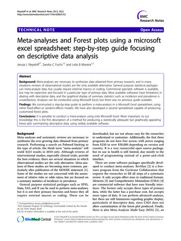
Neyeloff et al. BMC Research Notes 2012, 0* F2). Again, we multiply by 100 to have it inpercentage.3. In order to have each study in a different line, wewill assign ordinal numbers to the studies. Our effectsummary must be number 1 if we want it in the bottomof the graph. This is done manually in column H of ourspreadsheet.4. We are ready to build the graph. Insert Graph Scatter Plot. X values will be column I, lines 2-12, andY values column H, lines 2-12.5. We must now add the error bars. In Excel 2007 thisis done in the Layout tab, clicking the “Error Bar” button on the right side. In Excel 2003 we must right clickon the data series (points on the graph) and click “format data series”, then chose the “X error bar” tab. Inthis window we mark the option “personalized values”,and then assign columns J and K, lines 2 to 12, to thelower and upper value.6. To insert the line marking the summary effect valuewe will add another data series. First we manually buildthis data set in the spreadsheet. Then right click on thegraph Select Data. Click on “add”, and chose X valuesas column C, lines 15 to 26, and Y values as columns B,lines 15 to 26. A new set of points will appear on thegraph. Right-click on any of the new dots and select “format data series”. Then we will choose “no marker” and“solid line” on the Marker Options and Line Color tabs.7. We can now format the X axis, right-clicking on it.In our example we want it to begin on 10 and end on28, interval of 2 units. It is not our case, but if theresearcher is dealing with relative data, then “logarithmic scale” must be marked.8. The graph is ready. The user can format colors,outlines, shadows and sizes. In our example we changedthe summary effect to a diamond shape. This is done byselecting only one dot (double click) and then rightclicking it.Page 5 of 69. For presentation we recommend copying and pasting the graph over a table with study information (Figure 3).ConclusionWe have constructed a guide to aid researchers interested in meta-analyzing data using a spreadsheet. To thebest of our knowledge there is no prior step-by-stepapproach, but it should be noted that all formulas andmethodology were previously publicly available.The main limitation of analyzing data in a spreadsheetis the potential for errors by typing incorrect formulas.We believe that a step-by-step approach as those presented in this article with all formulas already incorporated in the excel format can help minimize thispossibility. The guide presented also does not handleadvanced analyses such as multiple regression. However,this is not frequently used in summarizing descriptivedata. All sensitivity analysis must be done manually,including and excluding each study of the effect summary calculations, but this limitation is also present inother softwares.Microsoft Excel is part of the Microsoft Office Package, and therefore it is not free of costs. However, forthose who already have the package, this use of Excelcould amplify its utility offering an alternative for customizing the graphic presentation of the forest plot.The main limitation of the forest plot is that all studies are represented by squares of the same size, insteadof proportional to study weight. We did not feel thiscould overshadow all other formatting possibilities, sincestudy weight can also be estimated by the confidenceinterval width.In conclusion, it is possible to meta-analyze data usinga Microsoft Excel spreadsheet, using either fixed effector random effects model. The main advantages of thisapproach are the understanding of the complete processFigure 3 Comparison of Forest Plots Comparison of forest plots produced using our spreadsheet (left) and CMA (right).
Neyeloff et al. BMC Research Notes 2012, 5:52http://www.biomedcentral.com/1756-0500/5/52and formulas, and the use of widely available software. Itis also possible and simple to make a forest plot usingexcel. Since displaying results in a graphically appealingbut also statistically correct way is usually a problem tomost researchers, we believe the method presented herecould be of great use. Figure 3 compares the graphobtained with our method and with CMA software.Availability and requirementsProject name: Meta-analyses and Forest Plots using aMicrosoft Excel spreadsheet: step-by-step guide focusingon descriptive data analysis;Project home page: none;Operating systems: any OS supporting MicrosoftExcel;Programming language: not-applicable;Other requirements: Microsoft Excel 2003 or higher;License: Creative Commons Attribution 3.0 Unported(CC BY 3.0);Restrictions to use by non-academics: noneAvailability of supporting dataThe spreadsheets mentioned and the CMA files used forcomparison of statistics are available as complementarymaterial.Additional materialAdditional file 1: Meta-analyses and forest plots in MS Excel. This filecontains both spreadsheets developed.Additional file 2: CMA calculations fixed effect. This is a portabledocument format (pdf) of the calculations performed by the softwareComprehensive Meta-Analysis, when calculating the effect summaryusing fixed effect model. It is provided so readers may compare thecalculations and results obtained using Microsoft Excel spreadsheet andthe commercial software.Page 6 of 6Competing interestsThe authors declare that they have no competing interests.Received: 4 August 2011 Accepted: 20 January 2012Published: 20 January 2012References1. Stroup DF, Berlin JA, Morton SC, et al: Meta-analysis of observationalstudies in epidemiology: a proposal for reporting. Meta-analysis OfObservational Studies in Epidemiology (MOOSE) group. JAMA 2000,283:2008-12.2. Copenhagen: The Nordic Cochrane Centre, The Cochrane Collaboration,2011. Review Manager (RevMan) [Computer program]. Version 5.1 [http://ims.cochrane.org/revman].3. Rosenberg M: MetaWin: Statistical Software for Meta-Analysis Version 2.Sunderland, Massachusetts: Sinauer Associates; 2000 [http://www.metawinsoft.com].4. Borenstein M, Hedges L, Higgins J, Rothstein H: Comprehensive Metaanalysis Version 2. Biostat, Englewood NJ; 2005 [http://www.meta-analysis.com].5. Bax L, Yu L-M, Ikeda N, et al: Development and validation of MIX:comprehensive free software for meta-analysis of causal research data.BMC Med Res Methodol 2006, 6:50.6. Eddy DM: FAST*PRO: Software for meta-analysis by the confidence profilemethod Academic Press; 1992.7. Wallace BC, Schmid CH, Lau J, et al: Meta-Analyst: software for metaanalysis of binary, continuous and diagnostic data. BMC Med ResMethodol 2009, 9:80.8. Borenstein M, Hedges LV, Higgins JPT, et al: Introduction to Meta-Analysis. 1edition. Wiley; 2009.9. Lipsey MW, Wilson D: Practical Meta-Analysis. 1 edition. Sage Publications,Inc; 2000.10. Egger M, Smith GD, Altman D: Systematic Reviews in Health Care: MetaAnalysis in Context. 2 edition. BMJ Books; 2001.11. Schriger DL, Altman DG, Vetter JA, et al: Forest plots in reports ofsystematic reviews: a cross-sectional study reviewing current practice. IntJ Epidemiol 2010, 39:421-9.12. Higgins JPT, Thompson SG, Deeks JJ, et al: Measuring inconsistency inmeta-analyses. BMJ 2003, 327:557-60.doi:10.1186/1756-0500-5-52Cite this article as: Neyeloff et al.: Meta-analyses and Forest plots usinga microsoft excel spreadsheet: step-by-step guide focusing ondescriptive data analysis. BMC Research Notes 2012 5:52.Additional file 3: CMA calculations random effects. This is a portabledocument format (pdf) of the calculations performed by the softwareComprehensive Meta-Analysis, when calculating the effect summaryusing random effects model. It is provided so readers may compare thecalculations and results obtained using Microsoft Excel spreadsheet andthe commercial software.AcknowledgementsThis study was funded by Conselho Nacional de Pesquisas (CNPq) andFundo de Incentivo à Pesquisa do Hospital de Clínicas de Porto Alegre (FIPEHCPA).Author detailsPost Graduate Program of Cardiology, Universidade Federal do Rio Grandedo Sul, Porto Alegre, Brazil. 2Hospital de Clínicas de Porto Alegre,Universidade Federal do Rio Grande do Sul, Porto Alegre, Brazil.1Submit your next manuscript to BioMed Centraland take full advantage of: Convenient online submission Thorough peer review No space constraints or color figure chargesAuthors’ contributionsJLN conceived the article, designed the spreadsheets, and drafted themanuscript. LBM and SCF revised the manuscript and approved the finalversion. Immediate publication on acceptance Inclusion in PubMed, CAS, Scopus and Google Scholar Research which is freely available for redistributionSubmit your manuscript atwww.biomedcentral.com/submit
TECHNICAL NOTE Open Access Meta-analyses and Forest plots using a microsoft excel spreadsheet: step-by-step guide focusing on descriptive data analysis Jeruza L Neyeloff1*, Sandra C Fuchs1,2 and Leila B Moreira1,2 Abstract Background: Meta-analyses are necessary to sy