Transcription
Proceedings of the 40th Annual Meeting of the Association forComputational Linguistics (ACL), Philadelphia, July 2002, pp. 360-367.BootstrappingSteven AbneyAT&T Laboratories – Research180 Park AvenueFlorham Park, NJ, USA, 07932AbstractThis paper refines the analysis of cotraining, defines and evaluates a newco-training algorithm that has theoretical justification, gives a theoretical justification for the Yarowsky algorithm, and shows that co-training andthe Yarowsky algorithm are based ondifferent independence assumptions.1OverviewThe term bootstrapping here refers to a problem setting in which one is given a small set oflabeled data and a large set of unlabeled data,and the task is to induce a classifier. The plenitude of unlabeled natural language data, andthe paucity of labeled data, have made bootstrapping a topic of interest in computationallinguistics. Current work has been spurred bytwo papers, (Yarowsky, 1995) and (Blum andMitchell, 1998).Blum and Mitchell propose a conditional independence assumption to account for the efficacy of their algorithm, called co-training, andthey give a proof based on that conditional independence assumption. They also give an intuitive explanation of why co-training works,in terms of maximizing agreement on unlabeled data between classifiers based on different“views” of the data. Finally, they suggest thatthe Yarowsky algorithm is a special case of theco-training algorithm.The Blum and Mitchell paper has been veryinfluential, but it has some shortcomings. Theproof they give does not actually apply directlyto the co-training algorithm, nor does it directlyjustify the intuitive account in terms of classifieragreement on unlabeled data, nor, for that matter, does the co-training algorithm directly seekto find classifiers that agree on unlabeled data.Moreover, the suggestion that the Yarowsky algorithm is a special case of co-training is basedon an incidental detail of the particular application that Yarowsky considers, not on the properties of the core algorithm.In recent work, (Dasgupta et al., 2001) provethat a classifier has low generalization error if itagrees on unlabeled data with a second classifierbased on a different “view” of the data. Thisaddresses one of the shortcomings of the originalco-training paper: it gives a proof that justifiessearching for classifiers that agree on unlabeleddata.I extend this work in two ways. First, (Dasgupta et al., 2001) assume the same conditionalindependence assumption as proposed by Blumand Mitchell. I show that that independence assumption is remarkably powerful, and violatedin the data; however, I show that a weaker assumption suffices. Second, I give an algorithmthat finds classifiers that agree on unlabeleddata, and I report on an implementation andempirical results.Finally, I consider the question of the relation between the co-training algorithm andthe Yarowsky algorithm. I suggest that theYarowsky algorithm is actually based on a different independence assumption, and I showthat, if the independence assumption holds, theYarowsky algorithm is effective at finding ahigh-precision classifier.2Problem Setting and NotationA bootstrapping problem consists of a spaceof instances X , a set of labels L, a function
Y : X L assigning labels to instances,and a space of rules mapping instances to labels. Rules may be partial functions; we writeF (x) if F abstains (that is, makes no prediction) on input x. “Classifier” is synonymouswith “rule”.It is often useful to think of rules and labelsas sets of instances. A binary rule F can bethought of as the characteristic function of theset of instances {x : F (x) }. Multi-classrules also define useful sets when a particulartarget class is understood. For any rule F ,we write F for the set of instances {x : F (x) }, or (ambiguously) for that set’s characteristicfunction.We write F̄ for the complement of F , eitheras a set or characteristic function. Note thatF̄ contains instances on which F abstains. Wewrite F for {x : F (x) 6 F (x) 6 }. WhenF does not abstain, F̄ and F are identical.Finally, in expressions like Pr[F Y ](with square brackets and “Pr”), the functionsF (x) and Y (x) are used as random variables.By contrast, in the expression P (F Y ) (withparentheses and “P ”), F is the set of instancesfor which F (x) , and Y is the set of instances for which Y (x) .3View IndependenceDefinition 1 A pair of views x1 , x2 satisfyview independence just in case: Pr[F u G v, Y y] Pr[F u Y y]and similarly for F H2 , G H1 . A classification problem instance satisfies rule independence just in case all opposing-view rule pairssatisfy rule independence.If instead of generating H1 and H2 from X1and X2 , we assume a set of features F (whichcan be thought of as binary rules), and takeH1 H2 F, rule independence reduces tothe Naive Bayes independence assumption.The following theorem is not difficult toprove; we omit the proof.Theorem 1 View independence implies ruleindependence.4Rule Independence andBootstrappingBlum and Mitchell’s paper suggests that rulesthat agree on unlabelled instances are useful inbootstrapping.Definition 3 Therules F and G isagreementratebetweenPr[F G F, G 6 ]Blum and Mitchell assume that each instance xconsists of two “views” x1 , x2 . We can take thisas the assumption of functions X1 and X2 suchthat X1 (x) x1 and X2 (x) x2 . They proposethat views are conditionally independent giventhe label.Pr[X1 x1 X2 x2 , Y y]Pr[X2 x2 X1 x1 , Y y]Definition 2 A pair of rules F H1 , G H2satisfies rule independence just in case, for allu, v, y:Pr[X1 x1 Y y]Pr[X2 x2 Y y]A classification problem instance satisfies viewindependence just in case all pairs x1 , x2 satisfyview independence.There is a related independence assumptionthat will prove useful. Let us define H1 to consist of rules that are functions of X1 only, anddefine H2 to consist of rules that are functionsof X2 only.Note that the agreement rate between rulesmakes no reference to labels; it can be determined from unlabeled data.The algorithm that Blum and Mitchell describe does not explicitly search for rules withgood agreement; nor does agreement rate playany direct role in the learnability proof given inthe Blum and Mitchell paper.The second lack is emended in (Dasguptaet al., 2001). They show that, if view independence is satisfied, then the agreement ratebetween opposing-view rules F and G upperbounds the error of F (or G). The followingstatement of the theorem is simplified and assumes non-abstaining binary rules.Theorem 2 For all F H1 , G H2 that satisfy rule independence and are nontrivial predictors in the sense that minu Pr[F u] Pr[F 6
G], one of the following inequalities holds:Y GPr[F 6 Y ] Pr[F 6 G]Pr[F̄ 6 Y ] Pr[F 6 G]If F agrees with G on all but ² unlabelled instances, then either F or F̄ predicts Y with error no greater than ². A small amount of labelled data suffices to choose between F and F̄ .I give a geometric proof sketch here; thereader is referred to the original paper for a formal proof. Consider figures 1 and 2. In thesediagrams, area represents probability. For example, the leftmost box (in either diagram) represents the instances for which Y , andthe area of its upper left quadrant representsPr[F , G , Y ]. Typically, in sucha diagram, either the horizontal or vertical lineis broken, as in figure 2. In the special case inwhich rule independence is satisfied, both horizontal and vertical lines are unbroken, as in figure 1.Theorem 2 states that disagreement upperbounds error. First let us consider a lemma, towit: disagreement upper bounds minority probabilities. Define the minority value of F givenY y to be the value u with least probabilityPr[F u Y y]; the minority probability is theprobability of the minority value. (Note thatminority probabilities are conditional probabilities, and distinct from the marginal probabilityminu Pr[F u] mentioned in the theorem.)In figure 1a, the areas of disagreement arethe upper right and lower left quadrants of eachbox, as marked. The areas of minority valuesare marked in figure 1b. It should be obviousthat the area of disagreement upper bounds thearea of minority values.The error values of F are the values oppositeto the values of Y : the error value is whenY and when Y . When minorityvalues are error values, as in figure 1, disagreement upper bounds error, and theorem 2 followsimmediately.However, three other cases are possible. Onepossibility is that minority values are oppositeto error values. In this case, the minority values of F̄ are error values, and disagreement between F and G upper bounds the error of F̄ . Y Y GG Y G FF (a) Disagreement(b) Minority ValuesFigure 1: Disagreement upper-bounds minorityprobabilities.This case is admitted by theorem 2. In thefinal two cases, minority values are the sameregardless of the value of Y . In these cases,however, the predictors do not satisfy the “nontriviality” condition of theorem 2, which requires that minu Pr[F u] be greater than thedisagreement between F and G.5The Unreasonableness of RuleIndependenceRule independence is a very strong assumption;one remarkable consequence will show just howstrong it is. The precision of a rule F is defined to be Pr[Y F ]. (We continue toassume non-abstaining binary rules.) If rule independence holds, knowing the precision of anyone rule allows one to exactly compute the precision of every other rule given only unlabeled dataand knowledge of the size of the target concept.Let F and G be arbitrary rules based on independent views. We first derive an expressionfor the precision of F in terms of G. Note thatthe second line is derived from the first by ruleindependence.P (F G)P (G F )P (Y F ) P (F GY )P (GY ) P (F GȲ )P (GȲ )P (F Y )P (GY ) P (F Ȳ )P (GȲ )P (Y F )P (G Y ) [1 P (Y F )]P (G Ȳ )P (G F ) P (G Ȳ )P (G Y ) P (G Ȳ )To compute the expression on the righthandside of the last line, we require P (Y G), P (Y ),P (G F ), and P (G). The first value, the precision of G, is assumed known. The second value,P (Y ), is also assumed known; it can at any ratebe estimated from a small amount of labeleddata. The last two values, P (G F ) and P (G),can be computed from unlabeled data.
Thus, given the precision of an arbitrary ruleG, we can compute the precision of any otherview rule F . Then we can compute the precisionof rules based on the same view as G by usingthe precision of some other-view rule F . Hencewe can compute the precision of every rule giventhe precision of any e 1: Some dataSome DataThe empirical investigations described here andbelow use the data set of (Collins and Singer,1999). The task is to classify names in textas person, location, or organization. There isan unlabeled training set containing 89,305 instances, and a labeled test set containing 289persons, 186 locations, 402 organizations, and123 “other”, for a total of 1,000 instances.Instances are represented as lists of features.Intrinsic features are the words making up thename, and contextual features are features ofthe syntactic context in which the name occurs. For example, consider Bruce Kaplan,president of Metals Inc. This text snippet contains two instances. The first has intrinsic features N:Bruce-Kaplan, C:Bruce, and C:Kaplan(“N” for the complete name, “C” for “contains”), and contextual feature M:president(“M” for “modified by”). The second instancehas intrinsic features N:Metals-Inc, C:Metals,C:Inc, and contextual feature X:president-of(“X” for “in the context of”).Let us define Y (x) if x is a “location”instance, and Y (x) otherwise. We can estimate P (Y ) from the test sample; it contains186/1000 location instances, giving P (Y ) .186.Let us treat each feature F as a rule predicting when F is present and otherwise. Theprecision of F is P (Y F ). The internal featureN:New-York has precision 1. This permits us tocompute the precision of various contextual features, as shown in the “Co-training” column ofTable 1. We note that the numbers do not evenlook like probabilities. The cause is the failureof view independence to hold in the data, combined with the instability of the estimator. (The“Yarowsky” column uses a seed rule to 25Y G F Y Y GG (a) Positive correlation Y G F (b) Negative correlationFigure 2: Deviation from conditional independence.P (Y F ), as is done in the Yarowsky algorithm,and the “Truth” column shows the true valueof P (Y F ).)7Relaxing the AssumptionNonetheless, the unreasonableness of view independence does not mean we must abandon theorem 2. In this section, we introduce a weakerassumption, one that is satisfied by the data,and we show that theorem 2 holds under thisweaker assumption.There are two ways in which the data can diverge from conditional independence: the rulesmay either be positively or negatively correlated, given the class value. Figure 2a illustrates positive correlation, and figure 2b illustrates negative correlation.If the rules are negatively correlated, thentheir disagreement (shaded in figure 2) is largerthan if they are conditionally independent, andthe conclusion of theorem 2 is maintained a fortiori. Unfortunately, in the data, they are positively correlated, so the theorem does not apply.Let us quantify the amount of deviation fromconditional independence. We define the conditional dependence of F and G given Y y to
be dy 1X Pr[G v Y y, F u] Pr[G v Y y] 2 u,v21baDefinition 4 Rules F and G satisfy weak ruledependence just in case, for y { , }:Figure 3: Positive correlation, Y .q1 p12p1 q1where p1 minu Pr[F u Y y], p2 minu Pr[G u Y y], and q1 1 p1 .By definition, p1 and p2 cannot exceed 0.5. Ifp1 0.5, then weak rule dependence reduces toindependence: if p1 0.5 and weak rule dependence is satisfied, then dy must be 0, which isto say, F and G must be conditionally independent. However, as p1 decreases, the permissibleamount of conditional dependence increases.We can now state a generalized version of theorem 2:Theorem 3 For all F H1 , G H2 thatsatisfy weak rule dependence and are nontrivialpredictors in the sense that minu Pr[F u] Pr[F 6 G], one of the following inequalitiesholds:Pr[F 6 Y ] Pr[F 6 G]Pr[F̄ 6 Y ] Pr[F 6 G]Consider figure 3. This illustrates the mostrelevant case, in which F and G are positivelycorrelated given Y . (Only the case Y isshown; the case Y is similar.) We assumethat the minority values of F are error values;the other cases are handled as in the discussionof theorem 2.Let u be the minority value of G when Y .In figure 3, a is the probability that G u whenF takes its minority value, and b is the probability that G u when F takes its majorityvalue.The value r a b is the difference. Notethat r 0 if F and G are conditionally independent given Y . In fact, we can show21If F and G are conditionally independent, thendy 0.This permits us to state a weaker version ofrule independence:dy p2p C qD r B Ap qthat r is exactly our measure dy of conditionaldependence:2dy a p2 b p2 (1 a) (1 p2 ) (1 b) (1 p2 ) a b a b 2rHence, in particular, we may write dy a b.Observe further that p2 , the minority probability of G when Y , is a weighted average ofa and b, namely, p2 p1 a q1 b. Combining thiswith the equation dy a b allows us to expressa and b in terms of the remaining variables, towit: a p2 q1 dy and b p2 p1 dy .In order to prove theorem 3, we need to showthat the area of disagreement (B C) upperbounds the area of the minority value of F (A B). This is true just in case C is larger than A,which is to say, if bq1 ap1 . Substituting ourexpressions for a and b into this inequality andsolving for dy yields:dy p2q1 p12p1 q1In short, disagreement upper bounds the minority probability just in case weak rule dependence is satisfied, proving the theorem.8The Greedy Agreement AlgorithmDasgupta, Littman, and McAllester suggest apossible algorithm at the end of their paper, butthey give only the briefest suggestion, and donot implement or evaluate it. I give here analgorithm, the Greedy Agreement Algorithm,
Input: seed rules F, Gloopfor each atomic rule HG’ G Hevaluate cost of (F,G’)keep lowest-cost G’if G’ is worse than G, quitswap F, G’10.8Precision0.6Figure 4: The Greedy Agreement Algorithmthat constructs paired rules that agree on unlabeled data, and I examine its performance.The algorithm is given in figure 4. It beginswith two seed rules, one for each view. At eachiteration, each possible extension to one of therules is considered and scored. The best one iskept, and attention shifts to the other rule.A complex rule (or classifier) is a list of atomicrules H, each associating a single feature h witha label . H(x) if x has feature h, andH(x) otherwise. A given atomic rule ispermitted to appear multiple times in the list.Each atomic rule occurrence gets one vote, andthe classifier’s prediction is the label that receives the most votes. In case of a tie, there isno prediction.The cost of a classifier pair (F, G) is basedon a more general version of theorem 2, thatadmits abstaining rules. The following theoremis based on (Dasgupta et al., 2001).Theorem 4 If view independence is satisfied,and if F and G are rules based on differentviews, then one of the following holds:Pr[F 6 Y F 6 ]Pr[F̄ 6 Y F̄ 6 ] δµ δδµ δwhere δ Pr[F 6 G F, G 6 ], and µ minu Pr[F u F 6 ].In other words, for a given binary rule F , a pessimistic estimate of the number of errors madeby F is δ/(µ δ) times the number of instanceslabeled by F , plus the number of instances leftunlabeled by F . Finally, we note that the costof F is sensitive to the choice of G, but the costof F with respect to G is not necessarily thesame as the cost of G with respect to F . To getan overall cost, we average the cost of F withrespect to G and G with respect to F .0.40.2000.20.40.60.81RecallFigure 5: Performance of the greedy agreementalgorithmFigure 5 shows the performance of the greedyagreement algorithm after each iteration. Because not all test instances are labeled (someare neither persons nor locations nor organizations), and because classifiers do not label allinstances, we show precision and recall ratherthan a single error rate. The contour lines showlevels of the F-measure (the harmonic mean ofprecision and recall). The algorithm is run toconvergence, that is, until no atomic rule canbe found that decreases cost. It is interestingto note that there is no significant overtraining with respect to F-measure. The final valuesare 89.2/80.4/84.5 recall/precision/F-measure,which compare favorably with the performanceof the Yarowsky algorithm (83.3/84.6/84.0).(Collins and Singer, 1999) add a special finalround to boost recall, yielding 91.2/80.0/85.2for the Yarowsky algorithm and 91.3/80.1/85.3for their version of the original co-training algorithm. All four algorithms essentially performequally well; the advantage of the greedy agreement algorithm is that we have an explanationfor why it performs well.9The Yarowsky AlgorithmFor Yarowsky’s algorithm, a classifier again consists of a list of atomic rules. The prediction ofthe classifier is the prediction of the first rule inthe list that applies. The algorithm constructs a
classifier iteratively, beginning with a seed rule.In the variant we consider here, one atomic ruleis added at each iteration. An atomic rule F ischosen only if its precision, Pr[G F ](as measured using the labels assigned by thecurrent classifier G), exceeds a fixed thresholdθ.1Yarowsky does not give an explicit justification for the algorithm. I show here that thealgorithm can be justified on the basis of twoindependence assumptions. In what follows, Frepresents an atomic rule under consideration,and G represents the current classifier. Recallthat Y is the set of instances whose true label is , and G is the set of instances {x : G(x) }.We write G for the set of instances labeled bythe current classifier, that is, {x : G(x) 6 }.The first assumption is precision independence.Definition 5 Candidate rule F and classifierG satisfy precision independence just in caseP (Y F , G ) P (Y F )A bootstrapping problem instance satisfies precision independence just in case all rules G andall atomic rules F that nontrivially overlap withG (both F G and F G are nonempty) satisfy precision independence.Precision independence is stated here so that itlooks like a conditional independence assumption, to emphasize the similarity to the analysisof co-training. In fact, it is only “half” an independence assumption—for precision independence, it is not necessary that P (Y F̄ , G ) P (Y F̄ ).The second assumption is that classifiersmake balanced errors. That is:P (Y , G F ) P (Y , G F )Let us first consider a concrete (but hypothetical) example. Suppose the initial classifiercorrectly labels 100 out of 1000 instances, andmakes no mistakes. Then the initial precision is1(Yarowsky, 1995), citing (Yarowsky, 1994), actuallyuses a superficially different score that is, however, amonotone transform of precision, hence equivalent toprecision, since it is used only for sorting.1 and recall is 0.1. Suppose further that we addan atomic rule that correctly labels 19 new instances, and incorrectly labels one new instance.The rule’s precision is 0.95. The precision ofthe new classifier (the old classifier plus the newatomic rule) is 119/120 0.99. Note that thenew precision lies between the old precision andthe precision of the rule. We will show that thisis always the case, given precision independenceand balanced errors.We need to consider several quantities: theprecision of the current classifier, P (Y G );the precision of the rule under consideration,P (Y F ); the precision of the rule on the current labeled set, P (Y F G ); and the precisionof the rule as measured using estimated labels,P (G F G ).The assumption of balanced errors impliesthat measured precision equals true precision onlabeled instances, as follows. (We assume herethat all instances have true labels, hence thatȲ Y .)P (F G Ȳ )P (F G Y ) P (F G Ȳ )P (F G )P (G F G ) P (F G Y )P (Y F G ) P (F G Y )P (Y F G )P (Y F G )This, combined with precision independence,implies that the precision of F as measuredon the labeled set is equal to its true precisionP (Y F ).Now consider the precision of the old and newclassifiers at predicting . Of the instances thatthe old classifier labels , let A be the number that are correctly labeled and B be thenumber that are incorrectly labeled. DefiningNt A B, the precision of the old classifieris Qt A/Nt . Let A be the number of newinstances that the rule under consideration correctly labels, and let B be the number that itincorrectly labels. Defining n A B, theprecision of the rule is q A/n. The precisionof the new classifier is Qt 1 (A A)/Nt 1 ,which can be written as:nNtQt qQt 1 Nt 1Nt 1That is, the precision of the new classifier isa weighted average of the precision of the oldclassifier and the precision of the new rule.
We have seen, then, that the Yarowsky algorithm, like the co-training algorithm, can be justified on the basis of an independence assumption, precision independence. It is important tonote, however, that the Yarowsky algorithm isnot a special case of co-training. Precision independence and view independence are distinctassumptions; neither implies the .60.81RecallFigure 6: Performance of the Yarowsky algorithmAn immediate consequence is that, if we onlyaccept rules whose precision exceeds a giventhreshold θ, then the precision of the new classifier exceeds θ. Since measured precision equalstrue precision under our previous assumptions,it follows that the true precision of the final classifier exceeds θ if the measured precision of every accepted rule exceeds θ.Moreover, observe that recall can be writtenas:NtA QtN N where N is the number of instances whose truelabel is . If Qt θ, then recall is boundedbelow by Nt θ/N , which grows as Nt grows.Hence we have proven the following theorem.Theorem 5 If the assumptions of precision independence and balanced errors are satisfied,then the Yarowsky algorithm with threshold θobtains a final classifier whose precision is atleast θ. Moreover, recall is bounded below byNt θ/N , a quantity which increases at eachround.Intuitively, the Yarowsky algorithm increasesrecall while holding precision above a thresholdthat represents the desired precision of the finalclassifier. The empirical behavior of the algorithm, as shown in figure 6, is in accordancewith this analysis.To sum up, we have refined previous work onthe analysis of co-training, and given a new cotraining algorithm that is theoretically justifiedand has good empirical performance.We have also given a theoretical analysis ofthe Yarowsky algorithm for the first time, andshown that it can be justified by an independence assumption that is quite distinct fromthe independence assumption that co-trainingis based on.ReferencesA. Blum and T. Mitchell. 1998. Combining labeledand unlabeled data with co-training. In COLT:Proceedings of the Workshop on ComputationalLearning Theory. Morgan Kaufmann Publishers.Michael Collins and Yoram Singer. 1999. Unsupervised models for named entity classification. InEMNLP.Sanjoy Dasgupta, Michael Littman, and DavidMcAllester. 2001. PAC generalization bounds forco-training. In Proceedings of NIPS.David Yarowsky. 1994. Decision lists for lexical ambiguity resolution. In Proceedings ACL 32.David Yarowsky. 1995. Unsupervised word sensedisambiguation rivaling supervised methods. InProceedings of the 33rd Annual Meeting of theAssociation for Computational Linguistics, pages189–196.2To see that view independence does not imply precision indepence, consider an example in which G Yalways. This is compatible with rule independence, butit implies that P (Y F G) 1 and P (Y F Ḡ) 0, violating precision independence.
training, defines and evaluates a new co-training algorithm that has theo-retical justification, gives a theoreti-cal justification for the Yarowsky algo-rithm, and shows that co-training and the Yarowsky algorithm are based on different independence assumptions.