Transcription
Industrial Engineering Design of Production Planning Systemsfor the Semiconductor IndustryProf. Robert C. LeachmanDept. of Industrial Engineering and Operations ResearchUniversity of California at BerkeleyMarch 2, 2013Production Planning refers to the business processes for establishing target schedules for theoutputs of factories, for scheduling the launch of new manufacturing lots in factories, fordetermining schedules for procurement of raw materials supporting new production, forscheduling the allocation and shipment of intermediate products for follow-on uses, and forquoting delivery dates in response to customer inquiries. Production planning is concerned withensuring on-time delivery of customer orders, with ensuring the raw materials needed to supportproduction are made available when required, and with determining the best deployment ofsupply-chain and manufacturing assets considering the available market opportunities. “Best” inthis sense embraces both maximum expected cash flow to the company as well as wisemanagement of the risks for excess inventory and lost sales.The business process for deciding changes to the asset base itself, i.e., purchase of newequipment, salvaging existing equipment, and increasing or decreasing staffing levels, is termedCapacity Planning, a related but different business process. Normally, the frequency of decisionmaking about changing the asset base is much less than the frequency of decision-making abouthow to deploy the assets. As we define it here, Capacity Planning precedes Production Planning,whereby Production Planning takes as given the asset base determined by the decisions made inCapacity Planning.Typically, the decisions of Production Planning are not expressed at a level of detail fullyenabling manufacturing and supply-chain execution. Instead, Production Planning provides goalsor targets and constraints for execution. A follow-on business process is required to enableexecution in manufacturing, termed Factory Floor Scheduling. Factory Floor Scheduling takesas given the decisions made in Production Planning concerning factory input schedules andtarget output schedules, the availability of raw materials, and the allocation and shipping ofintermediate products. Similarly, follow-on business processes may be required to fully enableshipments of intermediate products between supply-chain facilities, e.g., scheduling warehousetasks or dispatching individual transportation shipments.Figure 1 displays the databases and business processes embraced by Production Planning in acompany that manufactures its products. Starting in the upper right corner, customers engagewith an Order Entry and Delivery Quotation System. This system keeps track of supplycommitments to customers expressed as outstanding customer orders or as inventorycommitments. The outstanding customer orders plus internally generated orders for replenishingcontracted or targeted inventory levels are referred to as the Order Board. For a given productthat is sold, the portion of finished goods inventory and planned output of finished goods notcommitted to any customer is termed the Product Availability or the Available-to-Promisequantity. Customers submit requests for delivery quotes to this system. Delivery quotes arecalculated based on product availability. A time limit is attached to each quote; if the customer1
Figure 1. Information Flows in Production Planning erBoardQuotation &Order EntrySystemPrioritizeddemands andbuild usPlanningEngine(BPS)Queries ntsProductstructureandsourcingrulesFactory Plans(start and outschedules)2CustomerRawMaterialsSystemBill ofMaterialsSystem
accepts the quote and places an order (i.e., a commitment to buy the product on the quoteddelivery schedule) before the time limit, then the consumption of product availability isconfirmed. Otherwise, product supply tentatively reserved for the prospective customer is addedback to the product availability to support subsequent customer inquiries.At the upper left is a Demand Forecasting System, typically administered by the company’sMarketing department. This system prepares time-phased estimates of the unconstrained marketpotential (i.e., the potential sales at current prices, if product availability is forthcoming) for eachfinished good. An important input to the Demand Forecasting System is the Order Board. This isimportant for two reasons: (1) Orders represent real demand; that portion of demand is known.Forecasting effort is required only for the remaining portion of demand not yet realized. (2) It isvaluable to track the forecast errors for the various products. Demands for some products may bemuch easier to forecast than for others. Characterizing the relative uncertainty of demand forvarious products is helpful information for Production Planning. Ideally, the Quotation Systemshould record all customer requests for quotes as evidence of the existence of market demand,and furnish such information to the Forecasting System for the purposes of tracking forecasterrors. Short of that, the record of booked orders provides documentation of a subset of therealized demand.A second business function of the Demand Forecasting System is to electronically documentBuild Rules for each product. Build Rules specify how far through the supply-chain network thatproduction or procurement may be progressed without customer commitments in hand topurchase the finished goods resulting from that production or procurement. To implement BuildRules, each product or intermediate product in the supply chain is declared to be either “build toorder” (meaning production or procurement may not be started until a customer commitment isat hand), or “build to plan” (meaning production or procurement may proceed in response to thedemand forecast, regardless of whether or not customer orders fulfilling that forecast have beenreceived). This specification is internally consistent in the sense that a build-to-plan product isnever a follower of a build-to-order product in the product structure. The Build Rules also mayspecify a minimum inventory level for a build-to-plan intermediate product whose followers inthe product structure are build-to-order products. The consequent inventory of completed buildto-plan products should be the financial responsibility of the Marketing Department, not theManufacturing Department.A third business function of the Demand Forecasting System is to document prioritization of thevarious demands. The purpose of the priority scheme is to guide decisions to delay or deferfulfillment of demands when status and/or capabilities render it impossible to meet all demandson time. The total demand for each finished goods type in a given time period is stratified intomultiple priority classes, as will be discussed below.At the middle right is a Raw Materials System for managing the procurement and allocation ofraw materials used in production, typically administered by a Materials or Supply ChainDepartment. In particular, this system provides information concerning the availability of rawmaterials within vendor lead times.3
At the lower right is the Bill of Materials System, typically administered by the ProductEngineering department of the company. This system maintains in an electronically readableform the “wiring diagrams” of the required or acceptable intermediate products to be input to themanufacture of each finished goods type and each intermediate product. It also specifies thefactories or subcontractors qualified to fabricate or process each product.At the lower left are the Factory Databases administered by each Factory. These databasesspecify capacity, lead time and yield parameters for each product of each factory, as well asprovide status information on all work-in-process (WIP). To the extent that products may be intransit between factories, this set of databases also includes status information on goods-intransit as well as lead time parameters for interplant shipping. Status on any static inventory (i.e.,intermediate products or finished goods that are not WIP) also is provided by such systems.In the center of the figure is the Planning Engine. The Planning Engine is a pure application, inthe sense that no data concerning the company’s supply chain is maintained within the Engine.Instead, at run time, the Planning Engine retrieves build-rule, order board and demand forecastinputs from the Demand Forecasting System; WIP and inventory status and factory capabilitydata from the Factory Databases; product and process structure data from the BOM System; andraw materials availability data from the Raw Materials System. The output of the PlanningEngine includes (1) target input and output schedules for each product in each factory, fed to theappropriate Factory Databases, (2) allocation and shipping plans for disposition of factoryoutputs, also fed to the appropriate Factory Databases, (3) requests to procure raw materials fedto the Raw Materials System, and (4) revised product availability figures fed to the OrderQuotation System.A planning cycle is an exercise of the Planning Engine to update factory and shipping schedulesand to update the product available-to-promise quantities. We differentiate two types of planningcycles: In an incremental planning cycle, new demands are tendered to the Engine and theEngine is asked to prepare execution plans responding to those plans without changing theexecution plans that service demands previously tendered to the Engine. In a regenerativeplanning cycle (also known as a batch production cycle), all demands, new and previouslyknown, are tendered to the Engine for a complete re-planning of supply-chain execution.Any manufacturing business executes planning cycles addressing all the business functionsdescribed in Figure 1. But few have automated the planning cycle to the extent whereby theinputs needed to make a production plan are continuously maintained by the peripheral systems,and an automated production planning calculation may be initiated at any time. Notwithstandingcontemporary performance, that capability is taken as the engineering goal of designing andimplementing a production planning system.In principle, the same Planning Engine could be designed and used to execute incrementalplanning cycles or regenerative planning cycles; it is simply a matter of the particulars of the datathat are tendered to the Engine. In practice, almost every company performs at least some of eachkind of planning cycle, but depending on the nature of the business, one kind of cycle will bemore prevalent. Companies manufacturing many low-volume custom products tend to favorincremental planning cycles (because demand forecasting of custom products is impractical).4
Companies with very high capital investment in manufacturing facilities and marketopportunities exceeding the capabilities of that investment tend to favor regenerative planningcycles (to make sure the capital plant is always directed to generate maximum cash flow).The procedural elements of the Planning Engine are summarized in Figure 2. Demands for eachproduct are stratified by time and by priority class. These demand classes provide marketingmanagement’s input concerning the relative priorities of demands when it is impossible to fulfillall demands on time. Typically, the highest priority class consists solely of customercommitments. These demands are first priority, if on-time delivery is to be achieved. The excessof total demand forecast over booked customer commitments typically belongs to lower priorityclasses. These lower classes might be further subdivided into a class for replenishment of safetystocks protecting against supply-chain uncertainties or enabling immediate sales from inventory(so-called “turns business”), followed by a lower-priority class for the remainder of salesforecasts. In principle, there could be any number of priority classes; let R denote the number ofsuch classes.The first procedure of the Planning Engine is to carry out Requirements Planning. InRequirements Planning, static inventory and projected output from WIP are deducted fromdemands to determine what portion of demands requires new production, and on what late-aspossible input schedules, considering lead times, yields and product and process structure. This isdone for demand class 1, for the combination of demand classes 1 and 2, and so on until it isdone for combination of all R demand classes. That is, required factory input schedules to meetclass 1 demands on time, to meet classes 1 and 2 on time, etc., are determined. This is done forall products in all factories by means of a calculation working backwards through the supplychain network. If the product and process structure is simple, i.e., there are no alternative inputproducts or processes, then simple MRP (material requirements planning) logic may be applied.If not, optimization logic is required, as will be discussed later.The second procedure of the Planning Engine is Capacitated Loading. In Capacitated Loading,the equivalent requirements for factory input to meet prioritized demands as calculated byRequirements Planning are assessed relative to factory capacity. This requires optimization logic.The best possible factory input and output schedules are calculated, best in the sense that (1)Demand Class 1 is fulfilled as on-time as possible, (2) Subject to the service of Demand Class 1achieved in (1), Demand Class 2 is fulfilled as on-time as possible, and so on, until all R demandclasses are considered. Across the different products within the same demand class, rules ormetrics are required to prioritize them in the case that not all may be accommodated on time. Theanswer to Capacitated Loading consists of feasible input and target output schedules for everyproduct of every factory, as well as schedules for allocation and interplant shipping ofintermediate products. These answers are fed to the Factory Databases. Factory input schedulesrequiring raw materials not already in the supply chain are fed to the Raw Materials System sothat timely procurement of such materials may be planned.The last procedure of the Planning Engine is Availability Calculation. In the AvailabilityCalculation, customer commitments are deducted from the finished goods output plan calculatedby the Capacitated Loading procedure. The result is an updated statement of ProductAvailability, which is furnished to the Order Quotation System.5
Figure 2. Scope of Planning finished goodsinventoryFactory WIP-outprojections andstatic fety StockReplenishmentsSalesForecastsComputenet demands uteavailabilityfor quotationAvailability
Delivery Quotation and Calculation of AvailabilityThe procedures for updating availability as a function of changes in supply or changes incustomer commitments and for calculating best-feasible delivery quotes are readily explained asfollows. We suppose there is a discrete time grid of epochs t 1, 2, , T at which customerdeliveries may be scheduled, where T is the farthest-out epoch at which customer deliveryrequests will be entertained.It is most convenient to perform the analysis in terms of cumulative time histories of supply anddemand for each product. We illustrate the calculations for a single product, so the product indexon variables is suppressed. Let St, t 1, 2, , T denote the cumulative actual and plannedsupply of the product by time epoch. S1, the cumulative supply at time t 1, includes the currentfinished goods inventory of the product plus planned output of the product at time 1. Thecumulative supply at time 2 includes S1 plus planned output of the product at time 2, and so on.Let Ot, t 1, 2, , T denote the (cumulative) customer commitments for the product due at orbefore time t, t 1, 2, , T.The cumulative availability of the product at time t is denoted by At and is calculated asAt Min {Sτ Oτ τ t , t 1, , T } , t 1, 2, , T .(1)At represents the largest quantity of the product that may be promised to fulfill new customerorders requested at or before epoch t. Note that the minimization looks forward through timefrom epoch t in order to find the smallest difference between the cumulative supply andcumulative prior commitments in order to determine how much more supply is available topromise without disrupting service to previously placed orders.Now suppose a new customer request for a delivery quote is received. The customer request mayinclude multiple products; we shall concern ourselves here only with delivery requests for theproduct in question. Moreover, the customer’s request for the product in question may involvemultiple deliveries on multiple dates, whereby the customer wants as a response the best deliveryschedule that can be provided (but not earlier than requested). Let rt denote the quantity of theproduct requested for delivery at epoch t, t 1, 2, , T. (In a typical case, rt will be nonzero atonly one or several epochs.) We form the cumulative delivery request Rt calculated astRt rτ , t 1, 2, , T .τ 1We calculate the cumulative delivery quote asQt Min {At , Rt } , t 1, 2, , T .We then un-cumulate Qt to provide a quoted delivery schedule as follows:q1 Q1, qt Qt – Qt-1, t 2, 3, , T,7(2)
and we update the cumulative availability as follows:At Min {Aτ Qτ τ t , t 1, , T } , t 1, 2, , T .(3)We also should update the order board to (tentatively) include a reservation for the customerreflecting the quote provided, i.e.,Ot Ot Qt , t 1, 2, , T .If the customer rejects the quote or if the quote expires without the customer committing anorder, then the cumulative quote Qt should be deleted from the cumulative orders Ot, i.e.,Ot Ot Qt , t 1, 2, , T ,whereupon the cumulative availability should be recalculated as in (1).Numerical ExampleWe illustrate the foregoing formulas with the numerical example in Table 1. Suppose for aparticular product the finished goods inventory level is 120. The planned supply is 100 at epoch1, 100 at epoch 2, 120 at epoch 3, 120 at epoch 4, 120 at epoch 5, and 120 at epoch 6. Thisresults in the cumulative supply schedule shown in row 2 of the table. Suppose the deliveryschedules for previously accepted orders amount to 100 at epoch 1, 120 at epoch 2, 130 at epoch3, 105 at epoch 4, 150 at epoch 5, and 30 at epoch 6. This results in the cumulative ordersschedule shown in row 3 of the table. Row 4 simply differences these two time histories. Row 5applies the Min formula to establish the cumulative availability at each epoch. At or beforeepoch 5, not more than 75 can be promised to prospective customers, after which the availabilityrises to 165. Finally, suppose a customer request for a quote is received requesting deliveries of30 units at each of epochs 3, 4, 5 and 6. This results in the cumulative order request shown inrow 6 of the table. Taking a Min with row 5 (the cumulative availability) results in thecumulative delivery quote shown in row 7. This quote is un-cumulated in row 8. As shown inrow 8, the company’s best response to the customer’s inquiry is to offer 30 units at epochs 3 and4, but drop to only 15 units supplied at epoch 5, but then recover and deliver 45 units at epoch 6.Row 9 differences row 5 (the cumulative availability) and row 7 (the cumulative quote). In row10 the Min formula is applied to update the availability. In row 11 the cumulative orders areupdated to (tentatively) include the cumulative quote. Should the customer reject the quote orshould the quote expire, then a transaction is required to delete the quote from the orders. This isdone in row 12. Immediately following that transaction there should be another transaction torestore the availability. This is done by repeating the calculations in rows 4 and 5.8
Table 1. Illustration of Available-to-Promise and Delivery Quotation Calculations1. Time epoch2. Cum supply, St3. Cum orders, Ot4. Difference, 3. – 2.5. Cum availability At6. New order request Rt (cum)7. Delivery quote Qt (cum)8. Delivery quote qt9. Difference, 5. – 7.10. Revised At11. Revised Ot (rows 7 3)12. Revised Ot if no order (11 – 4545755635
Requirements PlanningThe standard calculus for computing material requirements, i.e., translating end-item demandsinto requirements for production of components and ordering of raw materials, is widely knownand widely available in software. (Hereafter, this calculus is termed “the MRP calculus.”)Certain restrictive assumptions about the product structure are required for the MRP calculus tobe applicable:-For any product, there are no alternatives for each of its predecessor components, i.e.,there cannot be any choice of components to input for the production of the givenproduct.-For any product, there cannot be a choice of manufacturing facilities to manufacture theproduct, i.e., the manufacturing source for the product is unique.If either of these conditions is not met, MRP calculus must be supplemented with other logic todecide among alternative sources.An additional concern is related to economics. Some product structures are characterized bybinning and substitution. For example, testing of a manufacturing lot may categorize productunits within the batch into various grades of quality or bins. The average fraction ofmanufacturing output ending up in a certain bin of quality is termed the bin split for that bin. Afollow-on product or customer sale may require a particular bin of quality or may accept any ofseveral bins of quality. In such a case, it may be unprofitable to accept all demands for low-binsplit items. If such demands were accepted, it would entail excessive production and excessivesupply of the other bins, far exceeding their demand. If economics is a concern, the MRPcalculus must be supplemented with other logic to decide whether or not to accept demands andpropagate the demands as material requirements.Requirements plans are most commonly prepared in terms of event-based schedules, i.e.,quantities to input or ship or procure by date. For repetitive volume manufacturing, an alternativemeans of expressing plans is in terms of rate-based schedules. In rate-based schedules, a timegrid of epochs is specified. Between consecutive epochs, the rates of material flows input intomanufacturing processes are required or assumed to be held constant. If we label the interval (t1, t] as “period t”, a decision variable xt indicates the rate of material flow scheduled duringperiod t. Software intended to generate event-based material requirements plans will schedulematerial quantities at specific delivery times, i.e., xt denotes the quantity of the material to bedelivered at epoch t. The software may be used to generate rate-based schedules if the decisionvariable xt is interpreted as the rate of flow during (t-1, t] rather than the quantity due oroccurring at epoch t. A challenge arises if rates of flow are desired to be held constant duringrelatively long periods such as weeks. In that case, the need for lead times to be integer in theMRP calculus presents a problem. Fortunately, the MRP calculus can be revised to admit noninteger lead times while generating rate-based schedules expressing constant rates of materialflow in the given intervals.10
Capacitated LoadingOnce new production requirements are determined, the next phase of the planning cycle concernsloading such requirements on factories in a feasible schedule of launches for production lots andthe consequent target output schedules. Process-based industries, such as petroleum refining,paper making, aluminum making or the like, have since the 1950s employed linear programmingoptimization calculations to make capacitated loading decisions. Such industries arecharacterized by a very capital-intensive resource carrying out continuous or near-continuousproduction governed by rate-based schedules. For such industries, linear programming or mixedinteger linear programming is a very good fit.Industries characterized by many stages of fabrication and assembly of many different kinds ofdiscrete parts in low-volumes or infrequent batches are much less amenable to accurate, practicalmodeling under the linear programming paradigm. Considering the large numbers of productsand inventory points involved, a precise mathematical programming model becomesimpractically large. In such industries the application of LP is rare. Instead, it is more commonfor approximate capacity analyses to be carried out using spreadsheets making calculations ofapproximate workloads on artificial, aggregate resources or some subset of important resources.Results of such spreadsheet analyses are the subject of discussion, review and iteration, and, as aresult, planning cycles are rarely automated in such industries.The semiconductor industry straddles the boundary between discrete parts manufacturing andprocess industry. Discrete manufacturing lots are progressed through many process steps infabrication, assembly and testing, yet fabrication plants are extremely capital-intensive. Thenumber of levels in the product structure is relatively small, and production volumes of products,or of families of products with similar capacity consumption, are high. Thus the numbers ofinventory points and products for capacity analysis are relatively low, rendering the capacitatedloading problem amenable to LP optimization.A special challenge presented by semiconductor manufacturing, and, for that matter, by allindustries utilizing planar fabrication process technology, is that the manufacturing process flowsare re-entrant. In wafer fabrication, multiple layers of circuitry are built up on the wafers,necessitating repeated visits to equipment interspersed with visits to other equipment. Thismeans new production lots must compete with work-in-process for capacity. Workloads onresources become functions of the time-histories of production lot launches. Considerablesophistication is required to generate an accurate yet practical linear programming formulation,as will be discussed below.Product Structure and Inventory vs. WIPIn general, there are choices that can be made when defining product and process structures andwhen establishing inventory points to de-couple manufacturing stages. Amenability of theplanning problem to formal optimization is seldom a criterion for consideration when suchstructures are defined. But it is an important consideration, as successful application of formal11
optimization enables much faster and more frequent planning cycles to be performed. Tominimize the number of inventory points, the following rule is suggested:1. If the next processing step does not require input of major raw materials or other products, andthe next step does not reduce the potential market for the product, then the product name shouldnot change at the next step and there should not be an inventory point before the next step.To understand this rule, note that portions of the overall manufacturing process may consist ofseries of processing steps in which no assembly or co-production occurs, and the product underproduction is not completed until the end of the series. The sequence of steps in the series istermed a process flow. A manufacturing lot of a given product passes through such a processflow without changing levels in the product structure. If at a certain step the potential market forthe lot is reduced, this means specialized processing is being performed to render the productsuitable for a certain subset of potential customers. A different choice of specialized processingon the manufacturing lot would make it suitable for a different subset of customers. This choicenecessitates a change of levels in the product structure, i.e., a change of product names. It may bedesirable to hold an inventory before the specialization point, especially if the build rules entailbuilding to plan before specialization and building to order afterwards. In this case, a corporateinventory point is defined just in front of the first specialization processing step.In typical practice, other inventory points may arise for administrative or jurisdictionalconvenience, permitting asynchronous scheduling of steps before and after such a point. Theseinventories are unnecessary from a production planning point of view. As a complement to theproduct and process structure as defined by rule 1 above, the following operational rule issuggested:2. Production activity between corporate inventory points is organized into process flowsoperated with rate-based schedules. Once production lots are launched into a process flow, theyare not eligible for re-scheduling until they reach the next corporate inventory point. That is,such lots must be kept moving according to target lead times. Moreover, production lots arescheduled to leave corporate inventory points only if workload and capacity permit progressingthe lots to the next corporate inventory point according to rate-based scheduling and target leadtimes.The rationale for this rule is illustrated in Figures 3 and 4. Figure 3 illustrates the case where rule2 is not enforced. A vicious cycle arises in the organizational dynamics. We could start theexplanation of this cycle at any point, but let us start in the upper left, where the sales departmentgenerates forecasts for the various products and informs manufacturing, which launchesproduction lots accordingly. Now suppose
Industrial Engineering Design of Production Planning Systems . for the Semiconductor Industry . . determining schedules for procurement of raw materials supporting new production, for scheduling the allocation and shipment of intermediate products for follow-on uses, and for . management of the ri