Transcription
This page intentionally left blank
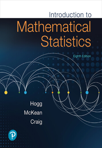
IntroductiontoMathematical StatisticsEighth EditionRobert V. HoggUniversity of IowaJoseph W. McKeanWestern Michigan UniversityAllen T. CraigLate Professor of StatisticsUniversity of Iowa
Director, Portfolio Management: Deirdre LynchCourseware Portfolio Manager: Patrick BarberaPortfolio Management Assistant: Morgan DannaContent Producer: Lauren MorseManaging Producer: Scott DisannoProduct Marketing Manager: Yvonne VannattaField Marketing Manager: Evan St. CyrMarketing Assistant: Jon BryantSenior Author Support/Technology Specialist: Joe VetereManager, Rights and Permissions: Gina CheselkaManufacturing Buyer: Carol Melville, LSC CommunicationsArt Director: Barbara AtkinsonProduction Coordination and Illustrations: IntegraCover Design: Studio MontageCover Image: Aleksandarvelasevic/Digital Vision Vectors/Getty Images.Copyright2019, 2013, 2005 by Pearson Education, Inc. All Rights Reserved. Printed in theUnited States of America. This publication is protected by copyright, and permission shouldbe obtained from the publisher prior to any prohibited reproduction, storage in a retrieval system, or transmission in any form or by any means, electronic, mechanical, photocopying, recording, or otherwise. For information regarding permissions, request forms and the appropriatecontacts within the Pearson Education Global Rights & Permissions department, please visitwww.pearsoned.com/permissions/.PEARSON and ALWAYS LEARNING are exclusive trademarks owned by Pearson Education,Inc. or its affiliates in the U.S. and/or other countries. Unless otherwise indicated herein, anythird-party trademarks that may appear in this work are the property of their respective ownersand any references to third-party trademarks, logos or other trade dress are for demonstrative ordescriptive purposes only. Such references are not intended to imply any sponsorship, endorsement,authorization, or promotion of Pearson’s products by the owners of such marks, or any relationshipbetween the owner and Pearson Education, Inc. or its affiliates, authors, licensees or distributors.Library of Congress Cataloging-in-Publications DataNames: Hogg, Robert V., author. McKean, Joseph W., 1944- author. Craig,Allen T. (Allen Thornton), 1905- author.Title: Introduction to mathematical statistics / Robert V. Hogg, Late Professor of Statistics,University of Iowa, Joseph W. McKean, Western Michigan University, Allen T. Craig,Late Professor of Statistics, University of Iowa.Description: Eighth edition. Boston : Pearson, [2019] Includesbibliographical references and index.Identifiers: LCCN 2017033015 ISBN 9780134686998 ISBN 0134686993Subjects: LCSH: Mathematical statistics.Classification: LCC QA276 .H59 2019 DDC 519.5–dc23 LC record available athttps://lccn.loc.gov/2017033015ISBN 13: 978-0-13-468699-8ISBN 10: 0-13-468699-3
Dedicated to my wife Margeand to the memory of Bob Hogg
This page intentionally left blank
ContentsPrefacexi1 Probability and Distributions1.1 Introduction . . . . . . . . . . . . . . . . . . . . . . . . . . . . .1.2 Sets . . . . . . . . . . . . . . . . . . . . . . . . . . . . . . . . .1.2.1 Review of Set Theory . . . . . . . . . . . . . . . . . . .1.2.2 Set Functions . . . . . . . . . . . . . . . . . . . . . . . .1.3 The Probability Set Function . . . . . . . . . . . . . . . . . . .1.3.1 Counting Rules . . . . . . . . . . . . . . . . . . . . . . .1.3.2 Additional Properties of Probability . . . . . . . . . . .1.4 Conditional Probability and Independence . . . . . . . . . . . .1.4.1 Independence . . . . . . . . . . . . . . . . . . . . . . . .1.4.2 Simulations . . . . . . . . . . . . . . . . . . . . . . . . .1.5 Random Variables . . . . . . . . . . . . . . . . . . . . . . . . .1.6 Discrete Random Variables . . . . . . . . . . . . . . . . . . . .1.6.1 Transformations . . . . . . . . . . . . . . . . . . . . . .1.7 Continuous Random Variables . . . . . . . . . . . . . . . . . .1.7.1 Quantiles . . . . . . . . . . . . . . . . . . . . . . . . . .1.7.2 Transformations . . . . . . . . . . . . . . . . . . . . . .1.7.3 Mixtures of Discrete and Continuous Type Distributions1.8 Expectation of a Random Variable . . . . . . . . . . . . . . . .1.8.1 R Computation for an Estimation of the Expected Gain1.9 Some Special Expectations . . . . . . . . . . . . . . . . . . . .1.10 Important Inequalities . . . . . . . . . . . . . . . . . . . . . . .1134712161823283137454749515356606568782 Multivariate Distributions2.1 Distributions of Two Random Variables . . .2.1.1 Marginal Distributions . . . . . . . . .2.1.2 Expectation . . . . . . . . . . . . . . .2.2 Transformations: Bivariate Random Variables2.3 Conditional Distributions and Expectations .2.4 Independent Random Variables . . . . . . . .2.5 The Correlation Coefficient . . . . . . . . . .2.6 Extension to Several Random Variables . . .85858993100109117125134v.
viContents2.72.82.6.1 Multivariate Variance-Covariance Matrix . . . . . . . . . . . 140Transformations for Several Random Variables . . . . . . . . . . . . 143Linear Combinations of Random Variables . . . . . . . . . . . . . . . 1513 Some Special Distributions3.1 The Binomial and Related Distributions . . . . . . . . .3.1.1 Negative Binomial and Geometric Distributions .3.1.2 Multinomial Distribution . . . . . . . . . . . . .3.1.3 Hypergeometric Distribution . . . . . . . . . . .3.2 The Poisson Distribution . . . . . . . . . . . . . . . . .3.3 The Γ, χ2 , and β Distributions . . . . . . . . . . . . . .3.3.1 The χ2 -Distribution . . . . . . . . . . . . . . . .3.3.2 The β-Distribution . . . . . . . . . . . . . . . . .3.4 The Normal Distribution . . . . . . . . . . . . . . . . . .3.4.1 Contaminated Normals . . . . . . . . . . . . . .3.5 The Multivariate Normal Distribution . . . . . . . . . .3.5.1 Bivariate Normal Distribution . . . . . . . . . . .3.5.2 Multivariate Normal Distribution, General Case3.5.3 Applications . . . . . . . . . . . . . . . . . . . .3.6 t- and F -Distributions . . . . . . . . . . . . . . . . . . .3.6.1 The t-distribution . . . . . . . . . . . . . . . . .3.6.2 The F -distribution . . . . . . . . . . . . . . . . .3.6.3 Student’s Theorem . . . . . . . . . . . . . . . . .3.7 Mixture Distributions . . . . . . . . . . . . . . . . . . 102122142184 Some Elementary Statistical Inferences4.1 Sampling and Statistics . . . . . . . . . . . . . . . . . . . . .4.1.1 Point Estimators . . . . . . . . . . . . . . . . . . . . .4.1.2 Histogram Estimates of pmfs and pdfs . . . . . . . . .4.2 Confidence Intervals . . . . . . . . . . . . . . . . . . . . . . .4.2.1 Confidence Intervals for Difference in Means . . . . . .4.2.2 Confidence Interval for Difference in Proportions . . .4.3 Confidence Intervals for Parameters of Discrete Distributions4.4 Order Statistics . . . . . . . . . . . . . . . . . . . . . . . . . .4.4.1 Quantiles . . . . . . . . . . . . . . . . . . . . . . . . .4.4.2 Confidence Intervals for Quantiles . . . . . . . . . . .4.5 Introduction to Hypothesis Testing . . . . . . . . . . . . . . .4.6 Additional Comments About Statistical Tests . . . . . . . . .4.6.1 Observed Significance Level, p-value . . . . . . . . . .4.7 Chi-Square Tests . . . . . . . . . . . . . . . . . . . . . . . . .4.8 The Method of Monte Carlo . . . . . . . . . . . . . . . . . . .4.8.1 Accept–Reject Generation Algorithm . . . . . . . . . .4.9 Bootstrap Procedures . . . . . . . . . . . . . . . . . . . . . .4.9.1 Percentile Bootstrap Confidence Intervals . . . . . . .4.9.2 Bootstrap Testing Procedures . . . . . . . . . . . . . .4.10 Tolerance Limits for Distributions . . . . . . . . . . . . . . 98303303308315.
Contentsvii5 Consistency and Limiting Distributions5.1 Convergence in Probability . . . . . . . . . . .5.1.1 Sampling and Statistics . . . . . . . . .5.2 Convergence in Distribution . . . . . . . . . . .5.2.1 Bounded in Probability . . . . . . . . .5.2.2 Δ-Method . . . . . . . . . . . . . . . . .5.2.3 Moment Generating Function Technique5.3 Central Limit Theorem . . . . . . . . . . . . .5.4 Extensions to Multivariate Distributions . . .3213213243273333343363413486 Maximum Likelihood Methods6.1 Maximum Likelihood Estimation . . . . .6.2 Rao–Cramér Lower Bound and Efficiency6.3 Maximum Likelihood Tests . . . . . . . .6.4 Multiparameter Case: Estimation . . . . .6.5 Multiparameter Case: Testing . . . . . . .6.6 The EM Algorithm . . . . . . . . . . . . 454461.7 Sufficiency7.1 Measures of Quality of Estimators . . . . . .7.2 A Sufficient Statistic for a Parameter . . . . .7.3 Properties of a Sufficient Statistic . . . . . . .7.4 Completeness and Uniqueness . . . . . . . . .7.5 The Exponential Class of Distributions . . . .7.6 Functions of a Parameter . . . . . . . . . . .7.6.1 Bootstrap Standard Errors . . . . . .7.7 The Case of Several Parameters . . . . . . . .7.8 Minimal Sufficiency and Ancillary Statistics .7.9 Sufficiency, Completeness, and Independence.8 Optimal Tests of Hypotheses8.1 Most Powerful Tests . . . . . . . . . . . . . . . . . . . . . . . . . . .8.2 Uniformly Most Powerful Tests . . . . . . . . . . . . . . . . . . . . .8.3 Likelihood Ratio Tests . . . . . . . . . . . . . . . . . . . . . . . . . .8.3.1 Likelihood Ratio Tests for Testing Means of Normal Distributions . . . . . . . . . . . . . . . . . . . . . . . . . . . . . .8.3.2 Likelihood Ratio Tests for Testing Variances of Normal Distributions . . . . . . . . . . . . . . . . . . . . . . . . . . . . .8.4 The Sequential Probability Ratio Test . . . . . . . . . . . . . . . . .8.5 Minimax and Classification Procedures . . . . . . . . . . . . . . . .8.5.1 Minimax Procedures . . . . . . . . . . . . . . . . . . . . . . .8.5.2 Classification . . . . . . . . . . . . . . . . . . . . . . . . . . .469469479487488495500507507510
viii9 Inferences About Normal Linear Models9.1 Introduction . . . . . . . . . . . . . . . . . . . .9.2 One-Way ANOVA . . . . . . . . . . . . . . . .9.3 Noncentral χ2 and F -Distributions . . . . . . .9.4 Multiple Comparisons . . . . . . . . . . . . . .9.5 Two-Way ANOVA . . . . . . . . . . . . . . . .9.5.1 Interaction between Factors . . . . . . .9.6 A Regression Problem . . . . . . . . . . . . . .9.6.1 Maximum Likelihood Estimates . . . . .9.6.2 Geometry of the Least Squares Fit . .9.7 A Test of Independence . . . . . . . . . . . . .9.8 The Distributions of Certain Quadratic Forms .9.9 The Independence of Certain Quadratic 56210 Nonparametric and Robust Statistics56910.1 Location Models . . . . . . . . . . . . . . . . . . . . . . . . . . . . . 56910.2 Sample Median and the Sign Test . . . . . . . . . . . . . . . . . . . . 57210.2.1 Asymptotic Relative Efficiency . . . . . . . . . . . . . . . . . 57710.2.2 Estimating Equations Based on the Sign Test . . . . . . . . . 58210.2.3 Confidence Interval for the Median . . . . . . . . . . . . . . . 58410.3 Signed-Rank Wilcoxon . . . . . . . . . . . . . . . . . . . . . . . . . . 58610.3.1 Asymptotic Relative Efficiency . . . . . . . . . . . . . . . . . 59110.3.2 Estimating Equations Based on Signed-Rank Wilcoxon . . . 59310.3.3 Confidence Interval for the Median . . . . . . . . . . . . . . . 59410.3.4 Monte Carlo Investigation . . . . . . . . . . . . . . . . . . . . 59510.4 Mann–Whitney–Wilcoxon Procedure . . . . . . . . . . . . . . . . . . 59810.4.1 Asymptotic Relative Efficiency . . . . . . . . . . . . . . . . . 60210.4.2 Estimating Equations Based on the Mann–Whitney–Wilcoxon 60410.4.3 Confidence Interval for the Shift Parameter Δ . . . . . . . . . 60410.4.4 Monte Carlo Investigation of Power . . . . . . . . . . . . . . 60510.5 General Rank Scores . . . . . . . . . . . . . . . . . . . . . . . . . . 60710.5.1 Efficacy . . . . . . . . . . . . . . . . . . . . . . . . . . . . . . 61010.5.2 Estimating Equations Based on General Scores . . . . . . . . 61210.5.3 Optimization: Best Estimates . . . . . . . . . . . . . . . . . . 61210.6 Adaptive Procedures . . . . . . . . . . . . . . . . . . . . . . . . . . 61910.7 Simple Linear Model . . . . . . . . . . . . . . . . . . . . . . . . . . . 62510.8 Measures of Association . . . . . . . . . . . . . . . . . . . . . . . . . 63110.8.1 Kendall’s τ . . . . . . . . . . . . . . . . . . . . . . . . . . . . 63110.8.2 Spearman’s Rho . . . . . . . . . . . . . . . . . . . . . . . . . 63410.9 Robust Concepts . . . . . . . . . . . . . . . . . . . . . . . . . . . . . 63810.9.1 Location Model . . . . . . . . . . . . . . . . . . . . . . . . . . 63810.9.2 Linear Model . . . . . . . . . . . . . . . . . . . . . . . . . . . 645
Contentsix11 Bayesian Statistics11.1 Bayesian Procedures . . . . . . . . . . .11.1.1 Prior and Posterior Distributions11.1.2 Bayesian Point Estimation . . .11.1.3 Bayesian Interval Estimation . .11.1.4 Bayesian Testing Procedures . .11.1.5 Bayesian Sequential Procedures .11.2 More Bayesian Terminology and Ideas .11.3 Gibbs Sampler . . . . . . . . . . . . . .11.4 Modern Bayesian Methods . . . . . . . .11.4.1 Empirical Bayes . . . . . . . . .655655656658662663664666672679682A Mathematical Comments687A.1 Regularity Conditions . . . . . . . . . . . . . . . . . . . . . . . . . . 687A.2 Sequences . . . . . . . . . . . . . . . . . . . . . . . . . . . . . . . . . 688B R PrimerB.1 Basics . . . . . . . . . . .B.2 Probability Distributions .B.3 R Functions . . . . . . . .B.4 Loops . . . . . . . . . . .B.5 Input and Output . . . .B.6 Packages . . . . . . . . . .693693696698699700700C Lists of Common Distributions703D Tables of Distributions707E References715F Answers to Selected Exercises721Index733
This page intentionally left blank
PrefaceWe have made substantial changes in this edition of Introduction to MathematicalStatistics. Some of these changes help students appreciate the connection betweenstatistical theory and statistical practice while other changes enhance the development and discussion of the statistical theory presented in this book.Many of the changes in this edition reflect comments made by our readers. Oneof these comments concerned the small number of real data sets in the previouseditions. In this edition, we have included more real data sets, using them toillustrate statistical methods or to compare methods. Further, we have made thesedata sets accessible to students by including them in the free R package hmcpkg.They can also be individually downloaded in an R session at the url listed below.In general, the R code for the analyses on these data sets is given in the text.We have also expanded the use of the statistical software R. We selected Rbecause it is a powerful statistical language that is free and runs on all three mainplatforms (Windows, Mac, and Linux). Instructors, though, can select anotherstatistical package. We have also expanded our use of R functions to computeanalyses and simulation studies, including several games. We have kept the level ofcoding for these functions straightforward. Our goal is to show students that witha few simple lines of code they can perform significant computations. Appendix Bcontains a brief R primer, which suffices for the understanding of the R used in thetext. As with the data sets, these R functions can be sourced individually at thecited url; however, they are also included in the package hmcpkg.We have supplemented the mathematical review material in Appendix A, placingit in the document Mathematical Primer for Introduction to Mathematical Statistics.It is freely available for students to download at the listed url. Besides sequences,this supplement reviews the topics of infinite series, differentiation, and integration (univariate and bivariate). We have also expanded the discussion of iteratedintegrals in the text. We have added figures to clarify discussion.We have retained the order of elementary statistical inferences (Chapter 4) andasymptotic theory (Chapter 5). In Chapters 5 and 6, we have written brief reviewsof the material in Chapter 4, so that Chapters 4 and 5 are essentially independentof one another and, hence, can be interchanged. In Chapter 3, we now begin thesection on the multivariate normal distribution with a subsection on the bivariatenormal distribution. Several important topics have been added. This includesTukey’s multiple comparison procedure in Chapter 9 and confidence intervals forthe correlation coefficients found in Chapters 9 and 10. Chapter 7 now contains axi
xiiPrefacediscussion on standard errors for estimates obtained by bootstrapping the sample.Several topics that were discussed in the Exercises are now discussed in the text.Examples include quantiles, Section 1.7.1, and hazard functions, Section 3.3. Ingeneral, we have made more use of subsections to break up some of the discussion.Also, several more sections are now indicated by as being optional.Content and Course PlanningChapters 1 and 2 develop probability models for univariate and multivariate variables while Chapter 3 discusses many of the most widely used probability models.Chapter 4 discusses statistical theory for much of the inference found in a standard statistical methods course. Chapter 5 presents asymptotic theory, concludingwith the Central Limit Theorem. Chapter 6 provides a complete inference (estimation and testing) based on maximum likelihood theory. The EM algorithm isalso discussed. Chapters 7–8 contain optimal estimation procedures and tests ofstatistical hypotheses. The final three chapters provide theory for three importanttopics in statistics. Chapter 9 contains inference for normal theory methods forbasic analysis of variance, univariate regression, and correlation models. Chapter10 presents nonparametric methods (estimation and testing) for location and univariate regression models. It also includes discussion on the robust concepts ofefficiency, influence, and breakdown. Chapter 11 offers an introduction to Bayesianmethods. This includes traditional Bayesian procedures as well as Markov ChainMonte Carlo techniques.Several courses can be designed using our book. The basic two-semester coursein mathematical statistics covers most of the material in Chapters 1–8 with topicsselected from the remaining chapters. For such a course, the instructor would havethe option of interchanging the order of Chapters 4 and 5, thus beginning the secondsemester with an introduction to statistical theory (Chapter 4). A one-semestercourse could consist of Chapters 1–4 with a selection of topics from Chapter 5.Under this option, the student sees much of the statistical theory for the methodsdiscussed in a non-theoretical course in methods. On the other hand, as with thetwo-semester sequence, after covering Chapters 1–3, the instructor can elect to coverChapter 5 and finish the course with a selection of topics from Chapter 4.The data sets and R functions used in this book and the R package hmcpkg canbe downloaded at the site:https://media.pearsoncmg.com/cmg/pmmg mml shared/mathstatsresources/home/index.html
PrefacexiiiAcknowledgementsBob Hogg passed away in 2014, so he did not work on this edition of the book.Often, though, when I was trying to decide whether or not to make a change in themanuscript, I found myself thinking of what Bob would do. In his memory, I haveretained the order of the authors for this edition.As with earlier editions, comments from readers are always welcomed and appreciated. We would like to thank these reviewers of the previous edition: JamesBaldone, Virginia College; Steven Culpepper, University of Illinois at UrbanaChampaign; Yuichiro Kakihara, California State University; Jaechoul Lee, BoiseState University; Michael Levine, Purdue University; Tingni Sun, University ofMaryland, College Park; and Daniel Weiner, Boston University. We appreciatedand took into consideration their comments for this revision. We appreciate thehelpful comments of Thomas Hettmansperger of Penn State University, Ash Abebeof Auburn University, and Professor Ioannis Kalogridis of the University of Leuven.A special thanks to Patrick Barbera (Portfolio Manager, Statistics), Lauren Morse(Content Producer, Math/Stats), Yvonne Vannatta (Product Marketing Manager),and the rest of the staff at Pearson for their help in putting this edition together.Thanks also to Richard Ponticelli, North Shore Community College, who accuracychecked the page proofs. Also, a special thanks to my wife Marge for her unwaveringsupport and encouragement of my efforts in writing this edition.Joe McKean
This page intentionally left blank
Chapter 1Probability and Distributions1.1IntroductionIn this section, we intuitively discuss the concepts of a probability model which weformalize in Secton 1.3 Many kinds of investigations may be characterized in partby the fact that repeated experimentation, under essentially the same conditions,is more or less standard procedure. For instance, in medical research, interest maycenter on the effect of a drug that is to be administered; or an economist may beconcerned with the prices of three specified commodities at various time intervals; oran agronomist may wish to study the effect that a chemical fertilizer has on the yieldof a cereal grain. The only way in which an investigator can elicit information aboutany such phenomenon is to perform the experiment. Each experiment terminateswith an outcome. But it is characteristic of these experiments that the outcomecannot be predicted with certainty prior to the experiment.Suppose that we have such an experiment, but the experiment is of such a naturethat a collection of every possible outcome can be described prior to its performance.If this kind of experiment can be repeated under the same conditions, it is calleda random experiment, and the collection of every possible outcome is called theexperimental space or the sample space. We denote the sample space by C.Example 1.1.1. In the toss of a coin, let the outcome tails be denoted by T and letthe outcome heads be denoted by H. If we assume that the coin may be repeatedlytossed under the same conditions, then the toss of this coin is an example of arandom experiment in which the outcome is one of the two symbols T or H; thatis, the sample space is the collection of these two symbols. For this example, then,C {H, T }.Example 1.1.2. In the cast of one red die and one white die, let the outcome be theordered pair (number of spots up on the red die, number of spots up on the whitedie). If we assume that these two dice may be repeatedly cast under the same conditions, then the cast of this pair of dice is a random experiment. The sample spaceconsists of the 36 ordered pairs: C {(1, 1), . . . , (1, 6), (2, 1), . . . , (2, 6), . . . , (6, 6)}.1
2Probability and DistributionsWe generally use small Roman letters for the elements of C such as a, b, orc. Often for an experiment, we are interested in the chances of certain subsets ofelements of the sample space occurring. Subsets of C are often called events and aregenerally denoted by capitol Roman letters such as A, B, or C. If the experimentresults in an element in an event A, we say the event A has occurred. We areinterested in the chances that an event occurs. For instance, in Example 1.1.1 wemay be interested in the chances of getting heads; i.e., the chances of the eventA {H} occurring. In the second example, we may be interested in the occurrenceof the sum of the upfaces of the dice being “7” or “11;” that is, in the occurrence ofthe event A {(1, 6), (2, 5), (3, 4), (4, 3), (5, 2), (6, 1), (5, 6), (6, 5)}.Now conceive of our having made N repeated performances of the random experiment. Then we can count the number f of times (the frequency) that theevent A actually occurred throughout the N performances. The ratio f /N is calledthe relative frequency of the event A in these N experiments. A relative frequency is usually quite erratic for small values of N , as you can discover by tossinga coin. But as N increases, experience indicates that we associate with the event Aa number, say p, that is equal or approximately equal to that number about whichthe relative frequency seems to stabilize. If we do this, then the number p can beinterpreted as that number which, in future performances of the experiment, therelative frequency of the event A will either equal or approximate. Thus, althoughwe cannot predict the outcome of a random experiment, we can, for a large valueof N , predict approximately the relative frequency with which the outcome will bein A. The number p associated with the event A is given various names. Sometimes it is called the probability that the outcome of the random experiment is inA; sometimes it is called the probability of the event A; and sometimes it is calledthe probability measure of A. The context usually suggests an appropriate choice ofterminology.Example 1.1.3. Let C denote the sample space of Example 1.1.2 and let B bethe collection of every ordered pair of C for which the sum of the pair is equal toseven. Thus B {(1, 6), (2, 5), (3, 4), (4, 3), (5, 2)(6, 1)}. Suppose that the dice arecast N 400 times and let f denote the frequency of a sum of seven. Suppose that400 casts result in f 60. Then the relative frequency with which the outcome60was in B is f /N 400 0.15. Thus we might associate with B a number p that isclose to 0.15, and p would be called the probability of the event B.Remark 1.1.1. The preceding interpretation of probability is sometimes referredto as the relative frequency approach, and it obviously depends upon the fact that anexperiment can be repeated under essentially identical conditions. However, manypersons extend probability to other situations by treating it as a rational measureof belief. For example, the statement p 25 for an event A would mean to themthat their personal or subjective probability of the event A is equal to 25 . Hence,if they are not opposed to gambling, this could be interpreted as a willingness ontheir part to bet on the outcome of A so that the two possible payoffs are in theratio p/(1 p) 25 / 35 23 . Moreover, if they truly believe that p 25 is correct,they would be willing to accept either side of the bet: (a) win 3 units if A occursand lose 2 if it does not occur, or (b) win 2 units if A does not occur and lose 3 if
1.2. Sets3it does. However, since the mathematical properties of probability given in Section1.3 are consistent with either of these interpretations, the subsequent mathematicaldevelopment does not depend upon which approach is used.The primary purpose of having a mathematical theory of statistics is to providemathematical models for random experiments. Once a model for such an experiment has been provided and the theory worked out in detail, the statistician may,within this framework, make inferences (that is, draw conclusions) about the random experiment. The construction of such a model requires a theory of probability.One of the more logically satisfying theories of probability is that based on theconcepts of sets and functions of sets. These concepts are introduced in Section 1.2.1.2SetsThe concept of a set or a collection of objects is usually left undefined. However,a particular set can be described so that there is no misunderstanding as to whatcollection of objects is under consideration. For example, the set of the first 10positive integers is sufficiently well described to make clear that the numbers 34 and14 are not in the set, while the number 3 is in the set. If an object belongs to aset, it is said to be an element of the set. For example, if C denotes the set of realnumbers x for which 0 x 1, then 34 is an element of the set C. The fact that334 is an element of the set C is indicated by writing 4 C. More generally, c Cmeans that c is an element of the set C.The sets that concern us are frequently sets of numbers. However, the languageof sets of points proves somewhat more convenient than that of sets of numbers.Accordingly, we briefly indicate how we use this terminology. In analytic geometryconsiderable emphasis is placed on the fact that to each point on a line (on whichan origin and a unit point have been selected) there corresponds one and only onenumber, say x; and that to each number x there corresponds one and only one pointon the line. This one-to-one correspondence between the numbers and points on aline enables us to speak, without misunderstanding, of the “point x” instead of the“number x.” Furthermore, with a plane rectangular coordinate system and with xand y numbers, to each symbol (x, y) there corresponds one and only one point in theplane; and to each point in the plane there corresponds but one such symbol. Hereagain, we may speak of the “point (x, y),” meaning the “ordered number
In this edition, we have included more real data sets, using them to illustrate statistical methods or to compare methods. . itinthedocumentMathematical Primer for Introduction toMathematical Statistics. It is freely available for students to download at the listed url. Besides sequences,
