Transcription
College TrigonometryVersion bπcCorrected EditionbyCarl Stitz, Ph.D.Lakeland Community CollegeJeff Zeager, Ph.D.Lorain County Community CollegeJuly 4, 2013
iiAcknowledgementsWhile the cover of this textbook lists only two names, the book as it stands today would simplynot exist if not for the tireless work and dedication of several people. First and foremost, we wishto thank our families for their patience and support during the creative process. We would alsolike to thank our students - the sole inspiration for the work. Among our colleagues, we wish tothank Rich Basich, Bill Previts, and Irina Lomonosov, who not only were early adopters of thetextbook, but also contributed materials to the project. Special thanks go to Katie Cimperman,Terry Dykstra, Frank LeMay, and Rich Hagen who provided valuable feedback from the classroom.Thanks also to David Stumpf, Ivana Gorgievska, Jorge Gerszonowicz, Kathryn Arocho, HeatherBubnick, and Florin Muscutariu for their unwaivering support (and sometimes defense) of thebook. From outside the classroom, we wish to thank Don Anthan and Ken White, who designedthe electric circuit applications used in the text, as well as Drs. Wendy Marley and Marcia Ballingerfor the Lorain CCC enrollment data used in the text. The authors are also indebted to the goodfolks at our schools’ bookstores, Gwen Sevtis (Lakeland CC) and Chris Callahan (Lorain CCC),for working with us to get printed copies to the students as inexpensively as possible. We wouldalso like to thank Lakeland folks Jeri Dickinson, Mary Ann Blakeley, Jessica Novak, and CorrieBergeron for their enthusiasm and promotion of the project. The administrations at both schoolshave also been very supportive of the project, so from Lakeland, we wish to thank Dr. Morris W.Beverage, Jr., President, Dr. Fred Law, Provost, Deans Don Anthan and Dr. Steve Oluic, and theBoard of Trustees. From Lorain County Community College, we wish to thank Dr. Roy A. Church,Dr. Karen Wells, and the Board of Trustees. From the Ohio Board of Regents, we wish to thankformer Chancellor Eric Fingerhut, Darlene McCoy, Associate Vice Chancellor of Affordability andEfficiency, and Kelly Bernard. From OhioLINK, we wish to thank Steve Acker, John Magill, andStacy Brannan. We also wish to thank the good folks at WebAssign, most notably Chris Hall,COO, and Joel Hollenbeck (former VP of Sales.) Last, but certainly not least, we wish to thankall the folks who have contacted us over the interwebs, most notably Dimitri Moonen and JoelWordsworth, who gave us great feedback, and Antonio Olivares who helped debug the source code.
Table of Contentsvii10 Foundations of Trigonometry10.1 Angles and their Measure . . . . . . . . . . . . . . . . . . . . . . . . . . .10.1.1 Applications of Radian Measure: Circular Motion . . . . . . . . .10.1.2 Exercises . . . . . . . . . . . . . . . . . . . . . . . . . . . . . . . .10.1.3 Answers . . . . . . . . . . . . . . . . . . . . . . . . . . . . . . . . .10.2 The Unit Circle: Cosine and Sine . . . . . . . . . . . . . . . . . . . . . . .10.2.1 Beyond the Unit Circle . . . . . . . . . . . . . . . . . . . . . . . .10.2.2 Exercises . . . . . . . . . . . . . . . . . . . . . . . . . . . . . . . .10.2.3 Answers . . . . . . . . . . . . . . . . . . . . . . . . . . . . . . . . .10.3 The Six Circular Functions and Fundamental Identities . . . . . . . . . . .10.3.1 Beyond the Unit Circle . . . . . . . . . . . . . . . . . . . . . . . .10.3.2 Exercises . . . . . . . . . . . . . . . . . . . . . . . . . . . . . . . .10.3.3 Answers . . . . . . . . . . . . . . . . . . . . . . . . . . . . . . . . .10.4 Trigonometric Identities . . . . . . . . . . . . . . . . . . . . . . . . . . . .10.4.1 Exercises . . . . . . . . . . . . . . . . . . . . . . . . . . . . . . . .10.4.2 Answers . . . . . . . . . . . . . . . . . . . . . . . . . . . . . . . . .10.5 Graphs of the Trigonometric Functions . . . . . . . . . . . . . . . . . . . .10.5.1 Graphs of the Cosine and Sine Functions . . . . . . . . . . . . . .10.5.2 Graphs of the Secant and Cosecant Functions . . . . . . . . . . .10.5.3 Graphs of the Tangent and Cotangent Functions . . . . . . . . . .10.5.4 Exercises . . . . . . . . . . . . . . . . . . . . . . . . . . . . . . . .10.5.5 Answers . . . . . . . . . . . . . . . . . . . . . . . . . . . . . . . . .10.6 The Inverse Trigonometric Functions . . . . . . . . . . . . . . . . . . . . .10.6.1 Inverses of Secant and Cosecant: Trigonometry Friendly Approach10.6.2 Inverses of Secant and Cosecant: Calculus Friendly Approach . . .10.6.3 Calculators and the Inverse Circular Functions. . . . . . . . . . . .10.6.4 Solving Equations Using the Inverse Trigonometric Functions. . .10.6.5 Exercises . . . . . . . . . . . . . . . . . . . . . . . . . . . . . . . .10.6.6 Answers . . . . . . . . . . . . . . . . . . . . . . . . . . . . . . . . .10.7 Trigonometric Equations and Inequalities . . . . . . . . . . . . . . . . . .10.7.1 Exercises . . . . . . . . . . . . . . . . . . . . . . . . . . . . . . . .10.7.2 Answers . . . . . . . . . . . . . . . . . . . . . . . . . . . . . . . . .11 Applications of Trigonometry11.1 Applications of Sinusoids . .11.1.1 Harmonic Motion .11.1.2 Exercises . . . . . .11.1.3 Answers . . . . . . .11.2 The Law of Sines . . . . . .11.2.1 Exercises . . . . . .11.2.2 Answers . . . . . . .11.3 The Law of Cosines . . . . 1. 881. 885. 891. 894. 896. 904. 908. 910
viii11.3.1 Exercises . . . . . . . . .11.3.2 Answers . . . . . . . . . .11.4 Polar Coordinates . . . . . . . . .11.4.1 Exercises . . . . . . . . .11.4.2 Answers . . . . . . . . . .11.5 Graphs of Polar Equations . . . .11.5.1 Exercises . . . . . . . . .11.5.2 Answers . . . . . . . . . .11.6 Hooked on Conics Again . . . . .11.6.1 Rotation of Axes . . . . .11.6.2 The Polar Form of Conics11.6.3 Exercises . . . . . . . . .11.6.4 Answers . . . . . . . . . .11.7 Polar Form of Complex Numbers11.7.1 Exercises . . . . . . . . .11.7.2 Answers . . . . . . . . . .11.8 Vectors . . . . . . . . . . . . . . .11.8.1 Exercises . . . . . . . . .11.8.2 Answers . . . . . . . . . .11.9 The Dot Product and Projection11.9.1 Exercises . . . . . . . . .11.9.2 Answers . . . . . . . . . .11.10 Parametric Equations . . . . . .11.10.1 Exercises . . . . . . . . .11.10.2 Answers . . . . . . . . . .IndexTable of 1100410071012102710311034104310451048105910631069
PrefaceThank you for your interest in our book, but more importantly, thank you for taking the time toread the Preface. I always read the Prefaces of the textbooks which I use in my classes becauseI believe it is in the Preface where I begin to understand the authors - who they are, what theirmotivation for writing the book was, and what they hope the reader will get out of reading thetext. Pedagogical issues such as content organization and how professors and students should bestuse a book can usually be gleaned out of its Table of Contents, but the reasons behind the choicesauthors make should be shared in the Preface. Also, I feel that the Preface of a textbook shoulddemonstrate the authors’ love of their discipline and passion for teaching, so that I come awaybelieving that they really want to help students and not just make money. Thus, I thank my fellowPreface-readers again for giving me the opportunity to share with you the need and vision whichguided the creation of this book and passion which both Carl and I hold for Mathematics and theteaching of it.Carl and I are natives of Northeast Ohio. We met in graduate school at Kent State Universityin 1997. I finished my Ph.D in Pure Mathematics in August 1998 and started teaching at LorainCounty Community College in Elyria, Ohio just two days after graduation. Carl earned his Ph.D inPure Mathematics in August 2000 and started teaching at Lakeland Community College in Kirtland,Ohio that same month. Our schools are fairly similar in size and mission and each serves a similarpopulation of students. The students range in age from about 16 (Ohio has a Post-SecondaryEnrollment Option program which allows high school students to take college courses for free whilestill in high school.) to over 65. Many of the “non-traditional” students are returning to school inorder to change careers. A majority of the students at both schools receive some sort of financialaid, be it scholarships from the schools’ foundations, state-funded grants or federal financial aidlike student loans, and many of them have lives busied by family and job demands. Some willbe taking their Associate degrees and entering (or re-entering) the workforce while others will becontinuing on to a four-year college or university. Despite their many differences, our studentsshare one common attribute: they do not want to spend 200 on a College Algebra book.The challenge of reducing the cost of textbooks is one that many states, including Ohio, are takingquite seriously. Indeed, state-level leaders have started to work with faculty from several of thecolleges and universities in Ohio and with the major publishers as well. That process will takeconsiderable time so Carl and I came up with a plan of our own. We decided that the bestway to help our students right now was to write our own College Algebra book and give it awayelectronically for free. We were granted sabbaticals from our respective institutions for the Spring
xPrefacesemester of 2009 and actually began writing the textbook on December 16, 2008. Using an opensource text editor called TexNicCenter and an open-source distribution of LaTeX called MikTex2.7, Carl and I wrote and edited all of the text, exercises and answers and created all of the graphs(using Metapost within LaTeX) for Version 0.9 in about eight months. (We choose to create atext in only black and white to keep printing costs to a minimum for those students who prefera printed edition. This somewhat Spartan page layout stands in sharp relief to the explosion ofcolors found in most other College Algebra texts, but neither Carl nor I believe the four-colorprint adds anything of value.) I used the book in three sections of College Algebra at LorainCounty Community College in the Fall of 2009 and Carl’s colleague, Dr. Bill Previts, taught asection of College Algebra at Lakeland with the book that semester as well. Students had theoption of downloading the book as a .pdf file from our website www.stitz-zeager.com or buying alow-cost printed version from our colleges’ respective bookstores. (By giving this book away forfree electronically, we end the cycle of new editions appearing every 18 months to curtail the usedbook market.) During Thanksgiving break in November 2009, many additional exercises writtenby Dr. Previts were added and the typographicalerrors found by our students and others were corrected. On December 10, 2009, Version 2 was released. The book remains free for download atour website and by using Lulu.com as an on-demand printing service, our bookstores are now ableto provide a printed edition for just under 19. Neither Carl nor I have, or will ever, receive anyroyalties from the printed editions. As a contribution back to the open-source community, all ofthe LaTeX files used to compile the book are available for free under a Creative Commons Licenseon our website as well. That way, anyone who would like to rearrange or edit the content for theirclasses can do so as long as it remains free.The only disadvantage to not working for a publisher is that we don’t have a paid editorial staff.What we have instead, beyond ourselves, is friends, colleagues and unknown people in the opensource community who alert us to errors they find as they read the textbook. What we gain in nothaving to report to a publisher so dramatically outweighs the lack of the paid staff that we haveturned down every offer to publish our book. (As of the writing of this Preface, we’ve had threeoffers.) By maintaining this book by ourselves, Carl and I retain all creative control and keep thebook our own. We control the organization, depth and rigor of the content which means we can resistthe pressure to diminish the rigor and homogenize the content so as to appeal to a mass market.A casual glance through the Table of Contents of most of the major publishers’ College Algebrabooks reveals nearly isomorphic content in both order and depth. Our Table of Contents shows adifferent approach, one that might be labeled “Functions First.” To truly use The Rule of Four,that is, in order to discuss each new concept algebraically, graphically, numerically and verbally, itseems completely obvious to us that one would need to introduce functions first. (Take a momentand compare our ordering to the classic “equations first, then the Cartesian Plane and THENfunctions” approach seen in most of the major players.) We then introduce a class of functionsand discuss the equations, inequalities (with a heavy emphasis on sign diagrams) and applicationswhich involve functions in that class. The material is presented at a level that definitely prepares astudent for Calculus while giving them relevant Mathematics which can be used in other classes aswell. Graphing calculators are used sparingly and only as a tool to enhance the Mathematics, notto replace it. The answers to nearly all of the computational homework exercises are given in the
xitext and we have gone to great lengths to write some very thought provoking discussion questionswhose answers are not given. One will notice that our exercise sets are much shorter than thetraditional sets of nearly 100 “drill and kill” questions which build skill devoid of understanding.Our experience has been that students can do about 15-20 homework exercises a night so we verycarefully chose smaller sets of questions which cover all of the necessary skills and get the studentsthinking more deeply about the Mathematics involved.Critics of the Open Educational Resource movement might quip that “open-source is where badcontent goes to die,” to which I say this: take a serious look at what we offer our students. Lookthrough a few sections to see if what we’ve written is bad content in your opinion. I see this opensource book not as something which is “free and worth every penny”, but rather, as a high qualityalternative to the business as usual of the textbook industry and I hope that you agree. If you haveany comments, questions or concerns please feel free to contact me at jeff@stitz-zeager.com or Carlat carl@stitz-zeager.com.Jeff ZeagerLorain County Community CollegeJanuary 25, 2010
xiiPreface
Chapter 10Foundations of Trigonometry10.1Angles and their MeasureThis section begins our study of Trigonometry and to get started, we recall some basic definitionsfrom Geometry. A ray is usually described as a ‘half-line’ and can be thought of as a line segmentin which one of the two endpoints is pushed off infinitely distant from the other, as pictured below.The point from which the ray originates is called the initial point of the ray.PA ray with initial point P .When two rays share a common initial point they form an angle and the common initial point iscalled the vertex of the angle. Two examples of what are commonly thought of as angles areQPAn angle with vertex P .An angle with vertex Q.However, the two figures below also depict angles - albeit these are, in some sense, extreme cases.In the first case, the two rays are directly opposite each other forming what is known as a straightangle; in the second, the rays are identical so the ‘angle’ is indistinguishable from the ray itself.QPA straight angle.The measure of an angle is a number which indicates the amount of rotation that separates therays of the angle. There is one immediate problem with this, as pictured below.
694Foundations of TrigonometryWhich amount of rotation are we attempting to quantify? What we have just discovered is thatwe have at least two angles described by this diagram.1 Clearly these two angles have differentmeasures because one appears to represent a larger rotation than the other, so we must label themdifferently. In this book, we use lower case Greek letters such as α (alpha), β (beta), γ (gamma)and θ (theta) to label angles. So, for instance, we haveαβOne commonly used system to measure angles is degree measure. Quantities measured in degreesare denoted by the familiar ‘ ’ symbol. One complete revolution as shown below is 360 , and partsof a revolution are measured proportionately.2 Thus half of a revolution (a straight angle) measures11 2 (360 ) 180 , a quarter of a revolution (a right angle) measures 4 (360 ) 90 and so on.One revolution 360 180 90 Note that in the above figure, we have used the small square ‘ ’ to denote a right angle, as iscommonplace in Geometry. Recall that if an angle measures strictly between 0 and 90 it is calledan acute angle and if it measures strictly between 90 and 180 it is called an obtuse angle.It is important to note that, theoretically, we can know the measure of any angle as long as we12The phrase ‘at least’ will be justified in short order.The choice of ‘360’ is most often attributed to the Babylonians.
10.1 Angles and their Measure695know the proportion it represents of entire revolution.3 For instance, the measure of an angle whichrepresents a rotation of 32 of a revolution would measure 32 (360 ) 240 , the measure of an angle11which constitutes only 12of a revolution measures 12(360 ) 30 and an angle which indicatesno rotation at all is measured as 0 .240 30 0 Using our definition of degree measure, we have that 1 represents the measure of an angle which1constitutes 360of a revolution. Even though it may be hard to draw, it is nonetheless not difficultto imagine an angle with measure smaller than 1 . There are two ways to subdivide degrees. Thefirst, and most familiar, is decimal degrees. For example, an angle with a measure of 30.5 would61represent a rotation halfway between 30 and 31 , or equivalently, 30.5 720of a full rotation. This 360 can be taken to the limit using Calculus so that measures like 2 make sense.4 The second wayto divide degrees is the Degree - Minute - Second (DMS) system. In this system, one degree isdivided equally into sixty minutes, and in turn, each minute is divided equally into sixty seconds.5In symbols, we write 1 600 and 10 6000 , from which it follows that 1 360000 . To convert ameasure of 42.125 to the DMS system, we start by noting that 42.125 42 0.125 . Converting0the partial amount of degrees to minutes, we find 0.125 60 7.50 70 0.50 . Converting the1 00 partial amount of minutes to seconds gives 0.50 6010 3000 . Putting it all together yields42.125 42 0.125 42 7.5042 70 0.5042 70 300042 70 3000On the other hand, to convert 117 150 4500 to decimal degrees, we first compute 150 1 1 4500 3600 80. Then we find0031 600 This is how a protractor is graded.Awesome math pun aside, this is the same idea behind defining irrational exponents in Section 6.1.5Does this kind of system seem familiar?4 1 4and
696Foundations of Trigonometry117 150 4500 117 150 4500 117 1 4 1 809381 80 117.2625 Recall that two acute angles are called complementary angles if their measures add to 90 .Two angles, either a pair of right angles or one acute angle and one obtuse angle, are calledsupplementary angles if their measures add to 180 . In the diagram below, the angles α and βare supplementary angles while the pair γ and θ are complementary angles.βθγαSupplementary AnglesComplementary AnglesIn practice, the distinction between the angle itself and its measure is blurred so that the sentence‘α is an angle measuring 42 ’ is often abbreviated as ‘α 42 .’ It is now time for an example.Example 10.1.1. Let α 111.371 and β 37 280 1700 .1. Convert α to the DMS system. Round your answer to the nearest second.2. Convert β to decimal degrees. Round your answer to the nearest thousandth of a degree.3. Sketch α and β.4. Find a supplementary angle for α.5. Find a complementary angle for β.Solution. 1. To convert 0 α to the DMS system, we start with 111.371 111 0.371 00 . Next we convert60600.371 1 22.260 . Writing 22.260 220 0.260 , we convert 0.260 10 15.600 . Hence,111.371 111 0.371 111 22.260111 220 0.260111 220 15.600111 220 15.600Rounding to seconds, we obtain α 111 220 1600 .
10.1 Angles and their Measure6972. To convert β to decimal degrees, we convert 280it all together, we have1 600 7 15and 17001 36000 17 3600 .Putting37 280 1700 37 280 17007 15134897 360037.471 37 17 36003. To sketch α, we first note that 90 α 180 . If we divide this range in half, we get90 α 135 , and once more, we have 90 α 112.5 . This gives us a pretty goodestimate for α, as shown below.6 Proceeding similarly for β, we find 0 β 90 , then0 β 45 , 22.5 β 45 , and lastly, 33.75 β 45 .Angle αAngle β4. To find a supplementary angle for α, we seek an angle θ so that α θ 180 . We getθ 180 α 180 111.371 68.629 .5. To find a complementary angle for β, we seek an angle γ so that β γ 90 . We getγ 90 β 90 37 280 1700 . While we could reach for the calculator to obtain anapproximate answer, we choose instead to do a bit of sexagesimal7 arithmetic. We firstrewrite 90 90 00 000 89 600 000 89 590 6000 . In essence, we are ‘borrowing’ 1 600from the degree place, and then borrowing 10 6000 from the minutes place.8 This yields,γ 90 37 280 1700 89 590 6000 37 280 1700 52 310 4300 .Up to this point, we have discussed only angles which measure between 0 and 360 , inclusive.Ultimately, we want to use the arsenal of Algebra which we have stockpiled in Chapters 1 through9 to not only solve geometric problems involving angles, but also to extend their applicability toother real-world phenomena. A first step in this direction is to extend our notion of ‘angle’ frommerely measuring an extent of rotation to quantities which can be associated with real numbers.To that end, we introduce the concept of an oriented angle. As its name suggests, in an oriented6If this process seems hauntingly familiar, it should. Compare this method to the Bisection Method introducedin Section 3.3.7Like ‘latus rectum,’ this is also a real math term.8This is the exact same kind of ‘borrowing’ you used to do in Elementary School when trying to find 300 125.Back then, you were working in a base ten system; here, it is base sixty.
698Foundations of Trigonometryangle, the direction of the rotation is important. We imagine the angle being swept out startingfrom an initial side and ending at a terminal side, as shown below. When the rotation iscounter-clockwise9 from initial side to terminal side, we say that the angle is positive; when therotation is clockwise, we say that the angle is negative.alinTermerTminalSideInitial SidedSieInitial SideA positive angle, 45 A negative angle, 45 At this point, we also extend our allowable rotations to include angles which encompass more thanone revolution. For example, to sketch an angle with measure 450 we start with an initial side,rotate counter-clockwise one complete revolution (to take care of the ‘first’ 360 ) then continuewith an additional 90 counter-clockwise rotation, as seen below.450 To further connect angles with the Algebra which has come before, we shall often overlay an anglediagram on the coordinate plane. An angle is said to be in standard position if its vertex isthe origin and its initial side coincides with the positive x-axis. Angles in standard position areclassified according to where their terminal side lies. For instance, an angle in standard positionwhose terminal side lies in Quadrant I is called a ‘Quadrant I angle’. If the terminal side of anangle lies on one of the coordinate axes, it is called a quadrantal angle. Two angles in standardposition are called coterminal if they share the same terminal side.10 In the figure below, α 120 and β 240 are two coterminal Quadrant II angles drawn in standard position. Note thatα β 360 , or equivalently, β α 360 . We leave it as an exercise to the reader to verify thatcoterminal angles always differ by a multiple of 360 .11 More precisely, if α and β are coterminalangles, then β α 360 · k where k is an integer.129‘widdershins’Note that by being in standard position they automatically share the same initial side which is the positive x-axis.11It is worth noting that all of the pathologies of Analytic Trigonometry result from this innocuous fact.12Recall that this means k 0, 1, 2, . . .10
10.1 Angles and their Measure699y43α 120 21 4 3 2 1 1β 240 1234x 2 3 4Two coterminal angles, α 120 and β 240 , in standard position.Example 10.1.2. Graph each of the (oriented) angles below in standard position and classify themaccording to where their terminal side lies. Find three coterminal angles, at least one of which ispositive and one of which is negative.1. α 60 2. β 225 3. γ 540 4. φ 750 Solution.1. To graph α 60 , we draw an angle with its initial side on the positive x-axis and rotate60 1counter-clockwise 360 6 of a revolution. We see that α is a Quadrant I angle. To find angleswhich are coterminal, we look for angles θ of the form θ α 360 · k, for some integer k.When k 1, we get θ 60 360 420 . Substituting k 1 gives θ 60 360 300 .Finally, if we let k 2, we get θ 60 720 780 . 52. Since β 225 is negative, we start at the positive x-axis and rotate clockwise 225360 8 ofa revolution. We see that β is a Quadrant II angle. To find coterminal angles, we proceed asbefore and compute θ 225 360 · k for integer values of k. We find 135 , 585 and495 are all coterminal with 225 .yy443322α 60 1 4 3 2 1 11234 21x 4 3 2 1 1β 225 234x 2 3 3 4 4α 60 in standard position.1β 225 in standard position.
700Foundations of Trigonometry3. Since γ 540 is positive, we rotate counter-clockwise from the positive x-axis. One fullrevolution accounts for 360 , with 180 , or 12 of a revolution remaining. Since the terminalside of γ lies on the negative x-axis, γ is a quadrantal angle. All angles coterminal with γ areof the form θ 540 360 · k, where k is an integer. Working through the arithmetic, wefind three such angles: 180 , 180 and 900 .4. The Greek letter φ is pronounced ‘fee’ or ‘fie’ and since φ is negative, we begin our rotation1clockwise from the positive x-axis. Two full revolutions account for 720 , with just 30 or 12of a revolution to go. We find that φ is a Quadrant IV angle. To find coterminal angles, wecompute θ 750 360 · k for a few integers k and obtain 390 , 30 and 330 .yγ 540 y44332211 4 3 2 1 11234x 4 3 2 1 1 2 2 3 3 4 4γ 540 in standard position.1234xφ 750 φ 750 in standard position.Note that since there are infinitely many integers, any given angle has infinitely many coterminalangles, and the reader is encouraged to plot the few sets of coterminal angles found in Example10.1.2 to see this. We are now just one step away from completely marrying angles with the realnumbers and the rest of Algebra. To that end, we recall this definition from Geometry.Definition 10.1. The real number π is defined to be the ratio of a circle’s circumference to itsdiameter. In symbols, given a circle of circumference C and diameter d,π CdWhile Definition 10.1 is quite possibly the ‘standard’ definition of π, the authors would be remissif we didn’t mention that buried in this definition is actually a theorem. As the reader is probablyaware, the number π is a mathematical constant - that is, it doesn’t matter which circle is selected,the ratio of its circumference to its diameter will have the same value as any other circle. Whilethis is indeed true, it is far from obvious and leads to a counterintuitive scenario which is exploredin the Exercises. Since the diameter of a circle is twice its radius, we can quickly rearrange theCequation in Definition 10.1 to get a formula more useful for our purposes, namely: 2π r
10.1 Angles and their Measure701This tells us that for any circle, the ratio of its circumference to its radius is also always constant;in this case the constant is 2π. Suppose now we take a portion of the circle, so instead of comparingthe entire circumference C to the radius, we compare some arc measuring s units in length to theradius, as depicted below. Let θ be the central angle subtended by this arc, that is, an anglewhose vertex is the center of the circle and whose determining rays pass through the endpoints o
I used the book in three sections of College Algebra at Lorain County Community College in the Fall of 2009 and Carl’s colleague, Dr. Bill Previts, taught a section of College Algebra at Lakeland with the book that semester as well. Students had the option of downloading the book as a .pdf