Transcription
Chapter 65The TRANSREG ProcedureChapter Table of ContentsOVERVIEW . . . . . . . . . . . . . . . . . . . . . . . . . . . . . . . . . . . 3369GETTING STARTED . . . . . . . . . . . . . . . . . . . . . . . . . . . . . . 3370Main-Effects ANOVA . . . . . . . . . . . . . . . . . . . . . . . . . . . . . 3370Detecting Nonlinear Relationships . . . . . . . . . . . . . . . . . . . . . . . 3373SYNTAX . . . . . . . . . . . .PROC TRANSREG StatementBY Statement . . . . . . . . .FREQ Statement . . . . . . .ID Statement . . . . . . . . .MODEL Statement . . . . . .OUTPUT Statement . . . . .WEIGHT Statement . . . . . 3376. 3376. 3379. 3380. 3380. 3380. 3402. 3412DETAILS . . . . . . . . . . . . . . . . . . . . . . . . . . . . . . .Model Statement Usage . . . . . . . . . . . . . . . . . . . . . . .Smoothing Splines . . . . . . . . . . . . . . . . . . . . . . . . .Missing Values . . . . . . . . . . . . . . . . . . . . . . . . . . .Missing Values, UNTIE, and Hypothesis Tests . . . . . . . . . . .Controlling the Number of Iterations . . . . . . . . . . . . . . . .Using the REITERATE Algorithm Option . . . . . . . . . . . . .Avoiding Constant Transformations . . . . . . . . . . . . . . . .Constant Variables . . . . . . . . . . . . . . . . . . . . . . . . .Convergence and Degeneracies . . . . . . . . . . . . . . . . . . .Implicit and Explicit Intercepts . . . . . . . . . . . . . . . . . . .Passive Observations . . . . . . . . . . . . . . . . . . . . . . . .Point Models . . . . . . . . . . . . . . . . . . . . . . . . . . . .Redundancy Analysis . . . . . . . . . . . . . . . . . . . . . . . .Optimal Scaling . . . . . . . . . . . . . . . . . . . . . . . . . . .OPSCORE, MONOTONE, UNTIE, and LINEAR TransformationsSPLINE and MSPLINE Transformations . . . . . . . . . . . . .Specifying the Number of Knots . . . . . . . . . . . . . . . . . .SPLINE, BSPLINE, and PSPLINE Comparisons . . . . . . . . .Hypothesis Tests . . . . . . . . . . . . . . . . . . . . . . . . . .Output Data Set . . . . . . . . . . . . . . . . . . . . . . . . . . . 3413. 3413. 3415. 3418. 3419. 3420. 3421. 3422. 3422. 3423. 3423. 3424. 3424. 3425. 3428. 3428. 3430. 3431. 3433. 3433. 3436
3368 Chapter 65. The TRANSREG ProcedureOUTTEST Output Data Set . . . . . . . . . . . . . . . .Computational Resources . . . . . . . . . . . . . . . . . .Solving Standard Least-Squares Problems . . . . . . . . .Using the DESIGN Output Option . . . . . . . . . . . . .Choice Experiments: DESIGN, NORESTOREMISSING,STANT Usage . . . . . . . . . . . . . . .ANOVA Codings . . . . . . . . . . . . . . . . . . . . . .Displayed Output . . . . . . . . . . . . . . . . . . . . . .ODS Table Names . . . . . . . . . . . . . . . . . . . . . . . . . . . . . . . . . . . . . . . . . . . . . . . . . . . . .NOZEROCON. . . . . . . . . . . . . . . . . . . . . . . . . . . . . . . . .EXAMPLES . . . . . . . . . . . . . . . . . . . . . . . . . . . . . . .Example 65.1 Using Splines and Knots . . . . . . . . . . . . . . . .Example 65.2 Nonmetric Conjoint Analysis of Tire Data . . . . . . .Example 65.3 Metric Conjoint Analysis of Tire Data . . . . . . . . .Example 65.4 Transformation Regression of Exhaust Emissions DataExample 65.5 Preference Mapping of Cars Data . . . . . . . . . . . . 3444. 3445. 3446. 3470. 3476. 3477. 3490. 3490. 3491. 3491. 3500. 3504. 3516. 3523REFERENCES . . . . . . . . . . . . . . . . . . . . . . . . . . . . . . . . . . 3528SAS OnlineDoc : Version 8
Chapter 65The TRANSREG ProcedureOverviewThe TRANSREG (transformation regression) procedure fits linear models, optionallywith spline and other nonlinear transformations, and it can be used to code experimental designs prior to their use in other analyses.The TRANSREG procedure fits many types of linear models, including ordinary regression and ANOVAmetric and nonmetric conjoint analysis (Green and Wind 1975; de Leeuw,Young, and Takane 1976)metric and nonmetric vector and ideal point preference mapping (Carroll 1972)simple, multiple, and multivariate regression with variable transformations(Young, de Leeuw, and Takane 1976; Winsberg and Ramsay 1980; Breimanand Friedman 1985)redundancy analysis (Stewart and Love 1968) with variable transformations(Israels 1984)canonical correlation analysis with variable transformations (van der Burg andde Leeuw 1983)response surface regression (Meyers 1976; Khuri and Cornell 1987) with variable transformationsThe data set can contain variables measured on nominal, ordinal, interval, and ratioscales (Siegel 1956). Any mix of these variable types is allowed for the dependentand independent variables. The TRANSREG procedure can transform nominal variables by scoring the categories to minimize squared error (Fisher1938), or they can be expanded into dummy variablesordinal variables by monotonically scoring the ordered categories so that orderis weakly preserved (adjacent categories can be merged) and squared error isminimized. Ties can be optimally untied or left tied (Kruskal 1964). Ordinalvariables can also be transformed to ranks.interval and ratio scale of measurement variables linearly or nonlinearly withspline (de Boor 1978; van Rijckevorsel 1982) or monotone spline (Winsbergand Ramsay 1980) transformations. In addition, smooth, logarithmic, exponential, power, logit, and inverse trigonometric sine transformations are available.Transformations produced by the PROC TRANSREG multiple regression algorithm,requesting spline transformations, are often similar to transformations produced by
3370 Chapter 65. The TRANSREG Procedurethe ACE smooth regression method of Breiman and Friedman (1985). However,ACE does not explicitly optimize a loss function (de Leeuw 1986), while PROCTRANSREG always explicitly optimizes a squared-error loss function.PROC TRANSREG extends the ordinary general linear model by providing optimalvariable transformations that are iteratively derived using the method of alternatingleast squares (Young 1981). PROC TRANSREG iterates until convergence, alternating finding least-squares estimates of the parameters of the model given the currentscoring of the data (that is, the current vectors)finding least-squares estimates of the scoring parameters given the current setof model parametersFor more background on alternating least-squares optimal scaling methods and transformation regression methods, refer to Young, de Leeuw, and Takane (1976), Winsberg and Ramsay (1980), Young (1981), Gifi (1990), Schiffman, Reynolds, andYoung (1981), van der Burg and de Leeuw (1983), Israels (1984), Breiman and Friedman (1985), and Hastie and Tibshirani (1986). (These are just a few of the manyrelevant sources.)Getting StartedThis section provides several examples that illustrate features of the TRANSREGprocedure.Main-Effects ANOVAThis example shows how to use the TRANSREG procedure to code and fit a maineffects ANOVA model. The input data set contains the dependent variables Y, factorsX1 and X2, and 11 observations. The following statements perform a main-effectsANOVA:title ’Introductory Main-Effects ANOVA Example’;data A;input Y X1 X2 ;datalines;8 a a7 a a4 a b3 a b5 b a4 b a2 b b1 b b8 c a7 c aSAS OnlineDoc : Version 8
Main-Effects ANOVA 33715 c b2 c b;*---Fit a Main-Effects ANOVA model with 1, 0, -1 coding. ---;proc transreg ss2;model identity(Y) class(X1 X2 / effects);output coefficients replace;run;*---Print TRANSREG output data set---;proc print label;format Intercept -- X2a 5.2;run;Introductory Main-Effects ANOVA ExampleThe TRANSREG ProcedureTRANSREG Univariate Algorithm Iteration History for -10.000000.000000.88144ConvergedAlgorithm converged.The TRANSREG Procedure Hypothesis Tests for Identity(Y)Univariate ANOVA Table Based on the Usual Degrees of FreedomSourceDFSum ofSquaresMeanSquareModelErrorCorrected t MSEDependent MeanCoeff Var0.978954.6666720.97739F ValuePr F19.830.0005R-SquareAdj R-Sq0.88140.8370Univariate Regression Table Based on the Usual Degrees of aDFCoefficientType IISum 261.3334.16716.66740.333Figure 65.1.MeanSquareF ValuePr FLabel261.3334.16716.66740.333272.704.3517.3942.09 .00010.07050.00310.0002InterceptX1 aX1 bX2 aANOVA Example Output from PROC TRANSREGSAS OnlineDoc : Version 8
3372 Chapter 65. The TRANSREG ProcedureThe iteration history in Figure 65.1 shows that the final R-Square of 0.88144 isreached on the first iteration.This is followed by ANOVA, fit statistics, and regression tables. PROC TRANSREGuses an effects (also called deviations from means or 0, 1, -1) coding in this example.The TRANSREG procedure produces the data set displayed in Figure 65.2.Introductory Main-Effects ANOVA ORESCORESCORESCORESCORESCORESCORESCORESCORESCOREM 0ROW11ROW12YY874354218752.Figure 1.001.001.004.67.X1 aX1 bX2 aabbaabbaabbOutput Data Set from PROC TRANSREGThe output data set has three kinds of observations, identified by values of – TYPE– . When – TYPE– ’SCORE’, the observation contains information on the dependent and independent variables as follows:– Y is the original dependent variable.– X1 and X2 are the independent classification variables, and the Interceptthrough X2 a columns contain the main effects design matrix that PROCTRANSREG creates. The variable names are Intercept, X1a, X1b, andX2a. Their labels are shown in the listing. When – TYPE– ’M COEFFI’, the observation contains coefficients of the final linear model.When – TYPE– ’MEAN’, the observation contains the marginal means.The observations with – TYPE– ’SCORE’ form the score partition of the data set,and the observations with – TYPE– ’M COEFFI’ and – TYPE– ’MEAN’ form thecoefficient partition of the data set.SAS OnlineDoc : Version 8
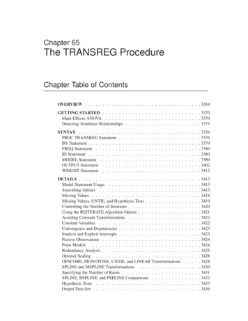
Detecting Nonlinear Relationships 3373Detecting Nonlinear RelationshipsThe TRANSREG procedure can detect nonlinear relationships among variables. Forexample, suppose 400 observations are generated from the following functiont x4 sin(x)and data are created as followsy t where is random normal error.The following statements find a cubic spline transformation of X with four knots. Forinformation on using splines and knots, see Example 65.1.The following statements produce Figure 65.3 through Figure 65.4:title ’Curve Fitting Example’;*---Create An Artificial Nonlinear Scatter Plot---;data Curve;Pi 3.14159265359;Pi4 4*Pi;Increment Pi4/400;do X Increment to Pi4 by Increment;T X/4 sin(X);Y T normal(7);output;end;run;*---Request a Spline Transformation of X---;proc transreg data Curve dummy;model identity(Y) spline(X / nknots 4);output predicted;id T;run;*---Plot the Results---;goptions goutmode replace nodisplay;%let opts haxis axis2 vaxis axis1 frame cframe ligr;* Depending on your goptions, these plot options may work better:* %let opts haxis axis2 vaxis axis1 frame;proc gplot;title;axis1 minor none label (angle 90 rotate 0);axis2 minor none;plot T*X 2/ &opts name ’tregin1’;plot Y*X 1/ &opts name ’tregin2’;SAS OnlineDoc : Version 8
3374 Chapter 65. The TRANSREG Procedureplot Y*X 1 T*X 2 PY*X 3 / &opts name ’tregin3’ overlay ;symbol1 color bluev star i none;symbol2 color yellow v none i join line 1;symbol3 color redv none i join line 2;run; quit;goptions display;proc greplay nofs tc sashelp.templt template l2r2;igout gseg;treplay 1:tregin1 2:tregin3 3:tregin2;run; quit;PROC TRANSREG increases the squared multiple correlation from the originalvalue of 0.19945 to 0.47062. The plot of T by X shows the original function, theplot of Y by X shows the error-perturbed data, and the third plot shows the data, thetrue function as a solid curve, and the regression function as the dashed curve. Theregression function closely approximates the true function.Curve Fitting ExampleThe TRANSREG ProcedureTRANSREG MORALS Algorithm Iteration History for 17ConvergedAlgorithm converged.Figure 65.3.SAS OnlineDoc : Version 8Curve Fitting Example Output
Detecting Nonlinear RelationshipsFigure 65.4. 3375Plots for the Curve Fitting ExampleSAS OnlineDoc : Version 8
3376 Chapter 65. The TRANSREG ProcedureSyntaxThe following statements are available in PROC TRANSREG.PROC TRANSREG DATA SAS-data-set OUTTEST SAS-data-set a-options o-options ;MODEL transform(dependents / t-options ) transform(dependents / t-options ). transform(independents / t-options ) transform(independents / t-options ). / a-options ;OUTPUT OUT SAS-data-set o-options ;ID variables ;FREQ variable ;WEIGHT variable ;BY variables ;To use the TRANSREG procedure, you need the PROC TRANSREG and MODELstatements. To produce an OUT output data set, the OUTPUT statement is required. PROC TRANSREG enables you to specify the same options in more thanone statement. All of the MODEL statement a-options (algorithm options) and all ofthe OUTPUT statement o-options (output options) can also be specified in the PROCTRANSREG statement. You can abbreviate all a-options, o-options, and t-options(transformation options) to their first three letters. This is a special feature of theTRANSREG procedure and is not generally true of other SAS/STAT procedures. SeeTable 65.1 on page 3377.The rest of this section provides detailed syntax information for each of the preceding statements, beginning with the PROC TRANSREG statement. The remainingstatements are described in alphabetical order.PROC TRANSREG StatementPROC TRANSREG DATA SAS-data-set OUTTEST SAS-data-set a-options o-options ;The PROC TRANSREG statement starts the TRANSREG procedure. Optionally,this statement identifies an input and an OUTTEST data set, specifies the algorithmand other computational details, requests displayed output, and controls the contentsof the OUT data set (which is created with the OUTPUT statement). The DATA and OUTTEST options can appear only in the PROC TRANSREG statement.The following table summarizes options available in the PROC TRANSREG statement. All a-options and o-options are described in the sections on either the MODELor OUTPUT statement, in which these options can also be specified.SAS OnlineDoc : Version 8
PROC TRANSREG StatementTable 65.1. 3377Options Available in the TRANSREG ProcedureTaskIdentify input data setspecifies input SAS data setOptionStatementDATA PROCOutput data set with test statisticsspecifies output test statistics data setOUTTEST PROCInput data setspecifies input observation typerestarts iterationsTYPE REITERATEMODELMODELSpecify method and control iterationsspecifies minimum criterion changespecifies minimum data changespecifies canonical dummy-variable initializationspecifies maximum number of iterationsspecifies iterative algorithmspecifies number of canonical variablesspecifies singularity criterionCCONVERGE CONVERGE DUMMYMAXITER METHOD NCAN SINGULAR MODELMODELMODELMODELMODELMODELMODELControl missing data handlingincludes monotone special missing valuesexcludes observations with missing valuesunties special missing valuesMONOTONE NOMISSUNTIE MODELMODELMODELControl intercept and CLASS variablesCLASS dummy variable name prefixCLASS dummy variable label prefixno intercept or centeringorder of class variable levelscontrols output of reference levelsCLASS dummy variable label separatorsCPREFIX LPREFIX NOINTORDER REFERENCE SEPARATORS MODELMODELMODELMODELMODELMODELControl displayed outputconfidence limits alphadisplays parameter estimate confidence limitsdisplays model specification detailsdisplays iteration historiessuppresses displayed outputsuppresses the iteration historiesdisplays regression resultsdisplays ANOVA tabledisplays conjoint part-worth utilitiesALPHA DELMODELMODELMODELMODELMODELMODELMODELControl standardizationfits additive modeldo not zero constant variablesspecifies transformation standardizationADDITIVENOZEROCONSTANTTSTANDARD MODELMODELMODELPredicted values, residuals, scoresoutputs canonical scoresoutputs individual confidence limitsCANONICALCLIOUTPUTOUTPUTSAS OnlineDoc : Version 8
3378 Chapter 65. The TRANSREG ProcedureTable 65.1.(continued)Taskoutputs mean confidence limitsspecifies design matrix codingoutputs leveragedoes not restore missing valuessuppresses output of scoresoutputs predicted valuesoutputs redundancy variablesoutputs residualsOptionCLMDESIGN Y TPUTOUTPUTOUTPUTOutput data set replacementreplaces dependent variablesreplaces independent variablesreplaces all Output data set coefficientsoutputs coefficientsoutputs ideal point coordinatesoutputs marginal meansoutputs redundancy analysis YOUTPUTOUTPUTOUTPUTOUTPUTOutput data set variable name prefixesdependent variable approximationsindependent variable approximationscanonical dependent variablesconservative individual lower CLcanonical independent variablesconservative-individual-upper CLconservative-mean-lower CLconservative-mean-upper CLMETHOD MORALS untransformed dependentliberal-individual-lower CLliberal-individual-upper CLliberal-mean-lower CLliberal-mean-upper CLresidualspredicted valuesredundancy variablestransformed dependentstransformed independentsADPREFIX AIPREFIX CDPREFIX CILPREFIX CIPREFIX CIUPREFIX CMLPREFIX CMUPREFIX DEPENDENT LILPREFIX LIUPREFIX LMLPREFIX LMUPREFIX RDPREFIX PPREFIX RPREFIX TDPREFIX TIPREFIX UTOUTPUTOutput data set macroscreates macro variablesMACROOUTPUTOutput data set detailsdependent and independent approximationscanonical correlation coefficientscanonical elliptical point coordinatecanonical point coordinatescanonical quadratic point UTPUTOUTPUTOUTPUTSAS OnlineDoc : Version 8
FREQ StatementTable 65.1. 3379(continued)Taskapproximations to transformed dependentsapproximations to transformed independentselliptical point coordinatespoint coordinatesquadratic point coordinatesmultiple regression UTPUTDATA SAS-data-setspecifies the SAS data set to be analyzed. If you do not specify the DATA option,PROC TRANSREG uses the most recently created SAS data set. The data set mustbe an ordinary SAS data set; it cannot be a special TYPE data set.OUTTEST SAS-data-setspecifies an output data set to contain hypothesis tests results. When you specifythe OUTTEST option, the data set contains ANOVA results. When you specify theSS2 a-option, regression tables are also output. When you specify the UTILITIESo-option, conjoint analysis part-worth utilities are also output.BY StatementBY variables ;You can specify a BY statement with PROC TRANSREG to obtain separate analyses on observations in groups defined
Example 65.2 Nonmetric Conjoint Analysis of Tire Data .3500 Example 65.3 Metric Conjoint Analysis of Tire Data . . .3504 Example 65.4 Transformation Regression of Exhaust Emissions Data .3516 Example65.5PreferenceMappingofCarsData.352