Transcription
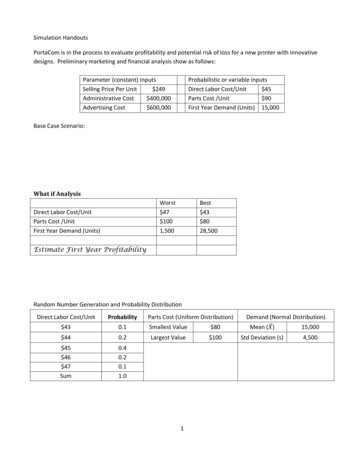
Simulation HandoutsPortaCom is in the process to evaluate profitability and potential risk of loss for a new printer with innovativedesigns. Preliminary marketing and financial analysis show as follows:Parameter (constant) InputsSelling Price Per Unit 249Administrative Cost 400,000Advertising Cost 600,000Probabilistic or variable inputsDirect Labor Cost/Unit 45Parts Cost /Unit 90First Year Demand (Units) 15,000Base Case Scenario:What if AnalysisWorst 47 1001,500Direct Labor Cost/UnitParts Cost /UnitFirst Year Demand (Units)Best 43 8028,500Estimate First Year ProfitabilityRandom Number Generation and Probability DistributionDirect Labor Cost/UnitProbabilityParts Cost (Uniform Distribution) 430.1Smallest Value 80 440.2Largest Value 100 45 46 47Sum0.40.20.11.01Demand (Normal Distribution)Mean ( )15,000Std Deviation (s)4,500
Summary Statistics2
Solution for PortaCom Example(Sim.xlsx/PortCom)3
Solutions to Summary StatisticsThe explanations of the following screen shots are given in the pages after these screen shots.Screen Shots for Data/Data Analysis/Histogram and Data/Data Analysis/Descriptive Statistics in Excel@4
The design of ProCom case simulation in Excel@Sim.xlsx/PortCom5
The output of Descriptive Statistics and Histogram:6
Now let us look at the whole process for the actual simulation of PorCom case:Procedures for Simulation (you may want to set Excel@ to manual calculations with MS Office Button / ExcelOptions / Formulas / Workbook Calculation / Manual and Press F9 whenever you need update calculations orsearch Excel@ Help with auto calculation to get detailed instructions) :1. Identify objectives and performance measures:a. Profitability as measured by Net Profit (SP – DL Cost – Part Cost) * Demand – Overhead Costb. Potential loss as measured by Probability of Loss No. of Losses/No. of Trials2. Set values for parameter or constant inputs:a. Selling Price 249b. Advertising cost 400,000c. Administrative cost 600,0003. Set Nt 600 from Cell E21 to Cell E620 , the number of replications equals toa. Ns 500 from Cell E121 to Cell 620, the number of replications to collect performance measuresb. Nw 100 from Cell E21 to Cell E120, the number of replications of warm up4. Calculate cumulative probabilities for Direct labor cost, and set up the table for From and To of randomnumbers, and Direct labor cost in three consecutive columns in the spreadsheet5. Set up the Trial numbers in Cells A21 to A620 with 1in Cell A21 and 600 in Cell A6206. Generate Month 1’s values of random variables ofa. Generate Direct labor cost per unit in Cell B21 with discrete probability distribution in Excel@with VLOOKUP(RAND(), A 10: C 14,3)b. Generate Part cost per unit in Cell C21 with uniform probability distribution in Excel@ with E 8 RAND()*( E 9- E 8)c. Generate Yearly Demand in Cell D21 with normal probability distribution in Excel@ with NORMINV(RAND(), E 13, E 14)7. Calculate Net Profit in Cell E21 in Excel@ with ( C 3-B21-C21)*D21- C 4- C 58. Verify the correctness of each formula very carefully9. Copy the formulas in the whole row 21 for Month 1 to rows 22 to row 620 or 599 rows of Nt10. Calculate Summary statistics in Excel@a. Click Data/Data Analysis/Descriptive Statistics,i. With the Input Range of Cells from E121 to E620 for Net Profits,ii. Select New Worksheet Ply with name as PorCom2,iii. Click options for both Summary Statistics and Confidence Interval 95% for the mean andclick OK to get the Descriptive Statistics Table in Worksheet PortCom2iv. You may format the values to make them more readablev. Results for Lower and Upper 95% Confidence Intervals are added. Please note theConfidence Interval (95%) in the output of Descriptive Statistics is the Margin of Error ort(α, n-1)* s/ , where t(α, n-1) TINV(0.05,n-1) or you may use t(α, n-1) 2 to get theapproximate 95% confidence interval for the mean.7
b. Use a range 3 million of Net Profits, use around 10 groups with a minimum from - 600,000 and agroup width of 300,000, to get Frequency Bin Ranges for Net Profits as in Cells H19 to H31.c. Click Data/Data Analysis/Histogram,i. With the Input Range of Cells from E121 to E620 for Net Profits,ii. With the Frequency Bin ranges in Cells H19 to H31,iii. Select New Worksheet Ply with name as PorCom3,iv. Click options Cumulative Percentage and Chart Output and click OK to see the results.11. Validate the results with real business operations and carefully study the logic of the simulation12. Analyze the results and provide recommendations13. Output Analysis for PortCom Case: (Refer to the Histogram, Frequency Distribution and the Table ofDescriptive Statistics on the next page)a. The estimate for the population mean Net Profit and its 95% confidence interval is given inDescriptive Statistics as follows:i. Mean ( ) 721,415 and its 95% confidence intervals are given by 0.05, 499 / from 674,204 to 768,627. Where The standard error / 24,029 and t(0.05, 499) 1.9647.The 9%% approximate 95% confidence intervals can be given by using 2 to replace t(0.05, 499).ii. How to interpret the approximate 95% confidence interval for the mean net profit? We are 95%sure that the unknown true population mean net profit is between 674,204 and 768,627 or ifwe construct 100 95% confidence intervals as we did for this one, over 95 out of the 100 CIswould contain the unknown true population mean net profit.b. The estimated probability of loss and its 95% confidence interval can be derived as follows:i. The probability of loss is given by the Cumulative % 9.20% when Net Profit is less than 0 ordivide 46, the number of replications of Net Profit less than 0, by Ns 500, the total number ofreplications in the simulation. ii. Use the equation 1 1 / to compute the 95% confidence interval from6.67% to 11.73% for the probability of loss, where z(0.975) 1.96, 0.092 and n 500.iii. How to interpret the 95% confidence interval for the probability of loss? We are 95% sure thatthe unknown true population proportion of loss is from 6.67% to 11.73% or if we construct 100such 95% confidence intervals for the probability of loss as we did for this one, over 95 out of the100 CIs would contain the unknown true population proportion of loss.c.What is the probability that the net profit will be more than 1.5 million?i. 100% - the cumulaive % for Net Profit less than 1.5 million or 93.6% 6.4%ii. The cumulative % for Net Profit less than 1.5 million is also shown in the Histogram as 93.6%.iii. A 95% confidence interval for the probabiltiy that the net profit will be more than 1.5 million canbe constructed in the same way as to construct the 95% CI for the probabiltiy of loss.8
(Anderson, Sweeney, Williams and Martin, 12e, pages 552 and 553Butler Electrical Supply Company (BESC) sales home ventilation fan for 125 per unit with the unit cost of 75.The monthly demand for the fan is normally distributed with a mean of 100 units and a standard deviation of 20units. BESC receives monthly delivery from its suppliers to replenish its inventory to a replenishment level of Q atthe beginning of each month. A 15 inventory holding cost is charged for each unit that is not sold when themonthly demand is less than the replenishment level Q. A 30 stock-out cost is charge for each unit of shortagewhen the monthly demand is greater than the replenishment level Q. The objectives of the simulation are toassess the monthly net profit resulting from using a particular replenishment level Q and to assess the servicelevel or the percentage of demand that will be satisfied.Controllable input is the replenishment level QThe probabilistic input is the monthly demand DOutput measures are the average monthly profit and the service level that equals to the ratio of total units sold tototal demand.Logics of Business Operations at Butler:Case 1: D Q.Gross Profit Holding Cost Net Profit Case 2: D Q.Gross Profit Shortage Cost Net Profit 9
10
Butler Class Exercise11
Butler Excel@ SImulationSim.xlsx/Butler12
Dynamic Simulation Models: Discrete –Event Simulation(Anderson, Sweeney, Williams and Martin, 12e, pages 557 and 560)Wachovia Bank has one automated teller machine (ATM) in each of its branch. The bank wants to assess whethermore than one ATM in each branch is necessary. The Bank established its service guidelines stating that theaverage waiting time for an ATM should be one minute or less.Assume: customers arrivals follow an uniform distribution (0, 4) or a RAND()* (b – a) RAND() * 4 and theATM service times follow normal distribution (2, 0.5) with a mean of 2 minutes and a standard deviation of 0.5minutes or NORMINV(RAND(),μ,σ) NORMINV(RAND(), 2, 0.5)Logics of Wachovia Bank One ATM Operations:Inter-arrival Time:Arrival Time:Service Start Time:Waiting Time:Service Time:Completion Time:Time in System:Inter-arrival times: randomly generated with Uniform (0, 4)Arrival time is the clock in time last arrival (Clock in)in Cell B21time current inter-arrival timeor in Cell C22: C21 B22Service start time the server available time:If the current Arrival time is late than the last Clock out (Completion) time,then the current Service start time the current Arrival time,else, the current Service start time the last completion timein Cell D22: MAX(C22, G21) or IF (C22 G21, C22, G21)Waiting time Service start time – Arrival timeIn Cell E22: D22 – C22Service time: randomly generated with Normal (2, 0.5)Completion time is the clock out time Service start time In system time Clock out (Completion) timeService time– Clock in(Arrival) time13
Wachovia Bank One ATM Class ExerciseSummary StatisticsNumber Waiting:Probability of Waiting:Average Waiting Time:Max Waiting Time:Utilization of ATM:Number Waiting 1 min:14
Solution to Class Exercise15
Wachovia Bank One ATM SimulationSim.xlsx/ATM16
Hungry Dawg Restaurants (Ragsdale, 5e Revised, page 563 with minor modifications in Excel@)As an analyst at Hungry Dawg, Lisa Pon is asked to determine how much money the company needs to accrue inthe coming year to pay for its employees’ health insurance claims. The company is self insured, meaning that itpays health insurance claims with its own money although it contracts with an outside company to handle theadministrative details of processing claims and writing checks. The money the company uses to pay claims comesfrom two sources: employee contributions or premiums deducted from employees’ paychecks, and companyfunds. The company must pay whatever costs are not covered by employee contributions. Each employeecovered by the health plan contributes 125 per month. However, the number of employees covered by the planchanges from month to month as employees are hired and fired, quit, or simply add or drop health insurancecoverage. A total of 18, 533 employees were covered by the plan last month. The average monthly health claimper covered employee was 250 last month.Hungry Dawg Restaurants Class Exercise (Rags12.xlsx/Figure12 2)1112121. What is the equation to compute Number of Employees for Month 1?Where:X0, X1, , and Xt Number of Covered Employees in Month 0, 1, , and t, respectively.rn the monthly rate of changes of the number of covered employees.In Excel@,2. What is the equation to compute Monthly Employee Contributions (MEC)?17
3. What is the equation to compute the Average Monthly Claim per Employee?Where:Y0, Y1, , and Yt Average Monthly Claim per Employee in Month 0, 1, , and t,respectively.rc the monthly rate of changes of the average claim per employee.In Excel@,4. What is the equation to compute the Monthly Total Claims (MTC)?5. What is the equation to compute the Monthly Company Cost (MCC)?In Excel@,6. What is the equation to compute the Total Company Cost (TCC)?The results of the first 12 months are given in the Figure 12.2 as follows (Rags12.xlsx/Fig12 2)Any change of any or all of these variables may lead to changes in Total Company Cost.18
Hungry Dawg Restaurants Class Exercise(Rags12.xlsx/Fig12 9Blank)19
Hungry Dawg Restaurants Final Version (Rags12.xlsx/Fig12 9WP)20
Topics to be covered:1. What is simulation and where simulation is used?2. Methods of Risk Analysisa. Best (most optimistic) case/worst (most pessimistic) case analysisb. What – if analysisc. Simulation3. Random Number Generationsa. General probability distribution with Probability Distribution Table. The Excel@VLOOKUP(RAND(),From To Value Arrays,3) is used to generate values of variables.b. Uniform distribution with a(lower limit) and b (upper limit). The following Excel@ formula is usedto generate values of uniform distributed random variables: a RAND() *(b-a)P(X x)P( X x) 1/(b – a)0ax a x a P( X x) (b a) a RAND () (b a)b axbXDemand (x) lower limit (a) RAND() (upper limit (b) – lower limit (a)) 5 RAND() (10 – 5)c. Poisson distribution with a mean arrival rate of λ. The following Excel@ formula is used togenerate values of inter-arrival times of Poisson distributed random variables: - 1/λ*LN(RAND())d. Exponential distribution with a mean service rate of μ. The following Excel@ formula is used togenerate values of service times of Exponential distributed random variables: - μ*LN(RAND())e. Bernoulli process with p as the probability of X 1 and 1 – p as the probability of X 0. Thefollowing Excel@ formula is used to generate values of Bernoulli process of random variables: if(RAND() p,1,0)21
f.Normal distribution with a mean of μ and a standard deviation of σ. The following Excel@formula is used to generate values of normal distributed random variables: NORMINV(RAND(), μ, σ) or μ NORMSINV(RAND())*σ * "# %'(&) , *, , ) ,- * / 0 * "# %&("2 3"' "# %("2 3"' , *, "# %&'(&) Sales (x) mean sales NORMSINV(RAND()) std sales 10 NORMSINV(RAND()) 2 NORMINV(RAND(), meanSales, StdSales) t/z table.html4. Simulation: Static (Monte Carlo) versus Dynamic (Discrete versus Continuous) Simulation5. Mathematical model4 5 6 , , , 8 Where 9 is the variable i in the model for i 1, 2, , kWhen the functional form of 5 is not known and/or the values of the parameters of β0, β1, , βk areknown or could not be found, simulation is one way to business decision making which evaluate theamount of reward and risk involved, the function of the uncertainty in the outcome of the decision andthe magnitude of the potential gain or in the decision.6. How to do simulation?a. Number of replications, over 100022
b. Data Analysis:i. Sample size (n)ii. Mean ( )iii. Standard deviation (s)iv.v.vi.vii.viii.Std Error ( ; ) s/ Min (Worst)Max (Best)(1-α)% CI for the true unknown population mean (μ): , 1 s/ (1-α)% CI for the true unknown population proportion (p): 1 1 / ix. Interpretation of the resultsc. Common used simulation software: SLAM, Crystal Balld. Verification and validation23
Procedures for Simulation (you may want to set Excel@ to manual calculations with MS Office Button / Excel Options / Formulas / Workbook Calculation / Manual and Press F9 whenever you need update calculations or search Excel@ Help with auto calculation to get detailed instructions) : 1. Identify objectives and performance measures: a.