WIXLIB

Lecture 34Fixed vs Random EffectsSTAT 512Spring 2011Background ReadingKNNL: Chapter 2534-1

Topic Overview Random vs. Fixed Effects Using Expected Mean Squares (EMS) toobtain appropriate tests in a Random orMixed Effects Model34-2

Fixed vs. Random Effects So far we have considered only fixed effectmodels in which the levels of each factorwere fixed in advance of the experimentand we were interested in differences inresponse among those specific levels. A random effects model considers factorsfor which the factor levels are meant to berepresentative of a general population ofpossible levels.34-3

Fixed vs. Random Effects (2) For a random effect, we are interested inwhether that factor has a significant effectin explaining the response, but only in ageneral way. If we have both fixed and random effects,we call it a “mixed effects model”. To include random effects in SAS, either usethe MIXED procedure, or use the GLMprocedure with a RANDOM statement.34-4

Fixed vs. Random Effects (2) In some situations it is clear from theexperiment whether an effect is fixed orrandom. However there are also situationsin which calling an effect fixed or randomdepends on your point of view, and onyour interpretation and understanding. Sosometimes it is a personal choice. Thisshould become more clear with someexamples.34-5

Random Effects Model This model is also called ANOVA II (orvariance components model). Here is the one-way model:Yij µ αi εijαi N (0, σA2 )εij N (0, σ2)Yij N (µ, σ σ2A independent 2)34-6

Random Effects Model (2)Now the cell means µi µ αi are randomvariables with a common mean. The question of“are they all the same” can now be addressed byconsidering whether the variance of theirdistribution is zero. Of course, the estimatedmeans will likely be at least slightly differentfrom each other; the question is whether thedifference can be explained by error variance σ 2alone.34-7

Two sources of variation Observations with the same i are dependent and2their covariance is σA .2A2 The components of variance are σ and σ . Wewant to get an idea of the relative magnitudes ofthese variance components. We often measure this by the intraclasscorrelation coefficient:σA222σA σ(correlation between two obs. with the same i)34-8

Parameters / ANOVA The cell means µij are now randomvariables, not parameters. The importantparameters are the variances σA2 and σ 2 The terms and layout of the ANOVA tableare the same as what we used for the fixedeffects model The expected mean squares (EMS) aredifferent because of the additional randomeffects, so we will estimate parameters in anew way.34-9

Parameters / ANOVA (2)2 E (MSE ) σ as usual. So we use MSE toestimate σ 22 For fixed effects, E (MSA) Q (A) σwhere Q(A) involves a l.c. of the αi . For random effects it becomesE (MSA) n σA2 σ 2 . From this you can2calculate that the estimate for σA should be(MSA MSE ) / n .34-10

Hypotheses Testing Our null hypothesis is that there is no effectof factor A. Under the random effectsmodel, it takes a different form:2H 0 : σA 02AHa : σ 0 For analysis of a single factor, the teststatistic is still F MSA/MSE with (r-1)and r(n-1) df. It WILL NOT remain thesame for multiple factors.34-11

ExampleKNNL Table 25.1 (page 1036)SAS code: applicant.sasY is the rating of a job applicantFactor A represents five different personnelinterviewers (officers), r 5 levels n 4 different applicants were randomlychosen and interviewed by eachinterviewer (i.e. 20 applicants); applicant isnot a factor since no applicant wasinterviewed more than once 34-12

Example (2) The interviewers were selected at randomfrom the pool of interviewers and hadapplicants randomly assigned. Here we are not so interested in thedifferences between the five interviewersthat happened to be picked (i.e. does Joegive higher ratings than Fred, is there adifference between Ethel and Bob). Ratherwe are interested in quantifying andaccounting for the effect of “interviewer” ingeneral.34-13

Example (3) There are other interviewers in the“population” and we want to makeinference about them too. Another way to say this is that with fixedeffects we are primarily interested in themeans of the factor levels (and differencesbetween them). With random effects, weare primarily interested in their variances.34-14

Plot of the Data34-15

34-16

SAS Codingproc glm data a1;class officer;model rating officer;random officer /test; Random statement is used and /test will performappropriate tests (and produce EMS)34-17

579.701099.252678.95MS394.92573.283F5.39Pr F0.0068Type III Expected Mean SquareVar(Error) 4 Var(Officer)SourceDFOfficer4Error: MS(Error) 15SS15801099MSF395 5.3973.3Pr F0.006834-18

Output (2) SAS gives us the EMS (note n 4replicates): E (MSA) σ 2 4σA2 SAS provides the appropriate test for eacheffect and tells you what “error term” isbeing used in testing. Note for thisexample it is as usual since there is onlyone factor.34-19

Variance Components VARCOMP procedure can be used to obtainthe variance components:proc varcomp data a1;class officer;model rating officer; Obtain point estimates of the two variances(could construct an estimate for the ICC)Variance 33334-20

Variance Components (2)2 SAS is providing σˆ 73.2833. Note thatthis is simply the MSE.2 SAS also indicates σˆofficer 80.4104 . Wecould calculate this from the mean squares:(MSA MSE ) (394.925 73.283) n4 VARCOMP procedure is somewhat limited(doesn’t provide ICC or SE’s)34-21

ICC The estimated intraclass correlationcoefficient isσˆA280.4104 0.523222σˆA σˆ80.4104 73.2833 About half the variance in rating isexplained by interviewer.34-22

MIXED Procedure Better than GLM / VARCOMP, but alsosomewhat more complex to use.Advantage is that it has optionsspecifically for mixed modelsproc mixed data a1 cl;class officer;model rating ;random officer /vcorr; Note: random effects are included ONLY inthe random statement; fixed effects in themodel statement. Different from GLM!34-23

Mixed Procedure The cl option after data a1 asks for theconfidence limits (on the variances). VCORR option provides the intraclasscorrelation coefficient. Have to watch out for huge amounts ofoutput – in this case there were 5 pages –we’ll just go through some of the pieces.34-24

OutputCov ParmofficerResidualEstimate80.4173.2895% CI24.46 149939.99 175.5Output from vcorr option (giving the ICC)Row Col11 1.00002 0.52323 0.52324 1.00000.5232Col40.52320.52320.52321.000034-25

Notes from Example Confidence intervals for variance components arediscussed in KNNL (pgs1041-1047) In this example, we would like the ICC to besmall, indicating that the variance due to theinterviewer is small relative to the variance due toapplicants. In many other examples, we may wantthis quantity to be large. What we found is that there is a significant effectof personnel officer (interviewer).34-26

Two Random FactorsYijk µ αi β j (αβ )ij εijkαi N (0, σ)2β j N (0, σB )2(αβ )ij N (0, σAB )2εij N (0, σ )2Yij N (µ, σA2 σB2 σAB σ2 )2A34-27

Two Random Factors (2)2µ Now the component σ can be divided upinto three components – A, B, and AB. There are five parameters in this model:2222µ, σA, σB , σAB , σ . Again, the cell means are random variables,not parameters!!!34-28

EMS for Two Random Factors22A22B2ABE (MSA) σ bn σ n σ2ABE (MSB ) σ an σ n σ2E (MSAB ) σ 2 n σABE (MSE ) σ 2 Estimates of the variance components can beobtained from these equations or other methods. Notice the patterns in the EMS: (these hold forbalanced data).34-29

Patterns in EMS2 They all contain σ . For MSA, also contain any variances with Ain subscript; similarly for MSB.2 The coefficient of σ is one; for any otherterm it is the product of n and all letters notrepresented in the subscript. (Can alsothink of it as the total number ofobservations at each fixed level of thecorresponding subscript – e.g. there are nbobservations for each level of A)34-30

Hypotheses Testing Testing based on EMS (apply null and look forratio of 1):2E (MSA) σ 2 bn σA2 n σAB2E (MSB ) σ 2 an σB2 n σAB2E (MSAB ) σ 2 n σABE (MSE ) σ 22 Test Interaction (H 0 : σAB 0 ) over error Test Main Effects (H 0 : σA2 0 and H 0 : σB2 0 )over interaction (this is the big difference!)34-31

Hypotheses Testing (Details)Main EffectsFactor A: H 0 : σA2 0 vs. H A : σA2 0Test Statistic: F MSA/MSAB – Denom is different!DF: (a-1) in num and (a-1)(b-1) in denomFactor B: H 0 : σB2 0 vs. H A : σB2 0Test Statistic: F MSB/MSAB – Denom is different!DF: (b-1) in num and (a-1)(b-1) in denom34-32

Hypotheses Testing (Details)Interaction22H 0 : σAB 0 vs. H A : σAB 0Test Statistic: F MSAB/MSE –Only for interaction is Denominator the MSEDF: (a-1)(b-1) in num and ab(n-1) in denom34-33

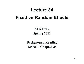
Example KNNL 25.15 (pg 1080) SAS code: mpg.sas Y is fuel efficiency in miles per gallon Factor A represents four different drivers,a 4 levels Factor B represents five different cars of thesame model , b 5 Each driver drove each car twice over thesame 40-mile test course (n 2)34-34

34-35

34-36

SAS Codingproc glm data a1;class driver car;model mpg driver car driver*car;random driver car driver*car/test;run;34-37

Output (1)Model and error outputSourceModelErrorCorrected TotalDF192039Sum ofSquares377.44475003.5150000380.9597500Factor effects outputSourceDFType I SSdriver3280.2847500car494.7135000driver*car 122.4465000Mean Square19.86551320.1757500Mean Square93.428250023.67837500.2038750F Value113.03F Value531.60134.731.16Pr F .0001Pr F .0001 .00010.3715Random statement outputSourceType III EMSdriverVar(Error) 2 Var(driver*car) 10 Var(driver)carVar(Error) 2 Var(driver*car) 8 Var(car)driver*car Var(Error) 2 Var(driver*car)34-38

Output (2)Note that only the interaction test is valid here:the test for interaction is MSAB/MSE, but thetests for main effects should be MSA/MSAB andMSB/MSAB which are done with the teststatement, not / MSE as is done here.Lesson: just because SAS spits out a P-value,doesn’t mean it is for a meaningful test!34-39

Output (3)Random/test outputThe GLM ProcedureTests of Hypotheses for Random Model Analysis of VarianceDependent Variable: mpgSource DF Type III or: MS(driver*car)Mean Square93.42825023.6783750.203875F Value458.26116.14Pr F .0001 .0001This last line says the denominator of the F tests is MSAB.Sourcedriver*carError: MS(Error)DF1220Type III SS2.4465003.515000Mean Square0.2038750.175750F Value1.16Pr F0.3715For the interaction term, the denominator is MSE (which isthe same test as was done above)34-40

Output (4)Proc varcompproc varcomp data efficiency;class driver car;model mpg driver car driver*car;MIVQUE(0) EstimatesVariance river*car)0.01406Var(Error)0.17575Can use Proc Mixed to get CI for variance components.34-41

Upcoming Two-Way Mixed Modelo One Fixed Effecto One Random Effect34-42

whether that factor has a significant effect in explaining the response, but only in a general way. . give higher ratings than Fred, is there a difference between Ethel and Bob). Rather we are interested in quantifying and accounting for the effect of “interviewer” in general. 34-14 Example (3) There are other interviewers in the “population” and we want to make inference about .