Transcription
Getting Started in R - StataNotes on Exploring Data(v. 1.0)Oscar Torres-Reynaotorres@princeton.eduFall 2010http://www.princeton.edu/ otorres/
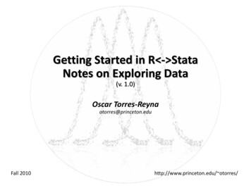
Tools for data analysis, a comparisonFeaturesLearningcurveSPSSSASStataJMP (SAS)RPython(Pandas)GradualPretty steepGradualGradualPretty steepSteepProgramming/Point-andProgramming point-andclickclickUser interfacePoint-andclickDatamanipulationStrongVery strongStrongStrongVery strongStrongData analysisVery strongVery strongVery strongStrongVery strongStrongGoodGoodVery goodVery goodExcellentGoodExpensive(perpetual,cost only withnew ual,cost only withnew amming ProgrammingOpen source Open source(free)(free)Free studentStudent disc.Student disc. version, 2014 Student disc.Released196819721985198919952008NOTE: The R content presented in this document is mostly based on an early version of Fox, J. and Weisberg, S. (2011) An R Companion to Applied Regression, SecondEdition, Sage; and from class notes from the ICPSR’s workshop Introduction to the R Statistical Computing Environment taught by John Fox during the summer of 2010.
This is the R screen in Multiple-Document Interface (MDI)
This is the R screen in Single-Document Interface (SDI)
Stata 12/13 screenVariables in dataset hereOutput hereHistory ofcommands, thiswindow?Files will besaved hereWrite commands hereProperty of eachvariable herePU/DSS/OTR
RStataWorking directorygetwd()# Shows the working directory (wd)setwd("C:/myfolder/data")# Changes the wdsetwd("H:\\myfolder\\data") # Changes the wdpwd/*Shows the working directory*/cd c:\myfolder\data/*Changes the wd*/cd “c:\myfolder\stata data” /*Notice the spaces*/Installing packages/user-written programsinstall.packages("ABC")# This will install thepackage –-ABC--. A window will pop-up, select amirror site to download from (the closest towhere you are) and click ok.library(ABC)# Load the package –-ABC-– to yourworkspace in Rssc install abc/*Will install the user-definedprogram ‘abc’. It will be ready to run.findit abc/*Will do an online search forprogram ‘abc’ or programs that include ‘abc’.It also searcher your computer.Getting help?plot # Get help for an object, in this case forthe –-plot– function. You can also type:help(plot)?regression # Search the help pages for anythingthat has the word "regression". You can alsotype: help.search("regression")apropos("age")# Search the word "age" in theobjects available in the current R session.help tab/* Get help on the command ‘tab’*/search regression/* Search the keywords for theword ‘regression’*/hsearch regression/* Search the help files forthe work ‘regression’. It provides more optionsthan ‘search’*/help(package car) # View documentation in package‘car’. You can also type:library(help "car“)help(DataABC)# Access codebook for a datasetcalled ‘DataABC’ in the package ABC6
RStataData from *.csv (copy-and-paste)# Select the table from the excel file, copy, goto the R Console and type:/* Select the table from the excel file, copy, goto Stata, in the command line type:mydata - read.table("clipboard", header TRUE,sep "\t")edit/*The data editor will pop-up and paste the data(Ctrl-V). Select the link for to include variablenamesData from *.csv# Reading the data directly/* In the command line type */mydata - read.csv("c:\mydata\mydatafile.csv",header TRUE)insheet using "c:\mydata\mydatafile.csv"# The will open a window to search for the *.csvfile.mydata - read.csv(file.choose(), header TRUE)/* Using the menu */Go to File- Import- ”ASCII data created byspreadsheet”. Click on ‘Browse’ to find the fileand then OK.Data from/to *.txt (space , tab, comma-separated)# In the example above, variables have spaces andmissing data is coded as ‘-9’mydata - read.table(("C:/myfolder/abc.txt",header TRUE, sep "\t", na.strings "-9")/* See insheet above */infile var1 var2 str7 var3 using abc.raw# Export the data/* Variables with embedded spaces must be enclosedin quotes */# Export datawrite.table(mydata, file "test.txt", sep "\t")outsheet using "c:\mydata\abc.csv"7
RStataData from/to SPSSinstall.packages("foreign")# Need to installpackage –-foreign–- first (you do this only once)./* Need to install the program ‘usespss’ (you dothis only once) */library(foreign) # Load package –-foreign--ssc install usespssmydata.spss a.sav",to.data.frame TRUE,use.value.labels TRUE,use.missings to.data.frame)/* To read the *.sav type (in one line):# Where:## ‘to.data.frame’ return a data frame.## ‘use.value.labels’ Convert variables with valuelabels into R factors with those levels.## ‘use.missings’ logical: should information onuser-defined missing values be used to set thecorresponding values to NA.Source: type ?read.spsshelp ------write.foreign(mydata, codefile "test2.sps",datafile "test2.raw", package “SPSS")# Provides a syntax file (*.sps) to read the *.rawdata fileusespss * For additional information type */Note: This does not work with SPSS portable -----------/* Stata does not convert files to SPSS. You needto save the data file as a Stata file version 9that can be read by SPSS v15.0 or later*//* From Stata type: */saveold mydata.dta/* Saves data to v.9 for SPSS8
RStataData from/to SAS# To read SAS XPORT format (*.xpt)library(foreign) # Load package –-foreign-mydata.sas ta.xpt") # Does not work for files onlinemydata.sas - read.xport("c:/myfolder/mydata.xpt")# Using package –-Hmisc—library(Hmisc)mydata ata.xpt)# It ----write.foreign(mydata, codefile "test2.sas",datafile "test2.raw", package “SAS")# Provide a syntax file (*.sas) to read the *.rawdata/*If you have a file in SAS XPORT format (*.xpt)you can use ‘fdause’ (or go to File- Import). */fdause "c:/myfolder/mydata.xpt“/* Type help fdause for more details *//* If you have SAS installed in your computer youcan use the program ‘usesas’, which you caninstall by typing: */ssc install usesas/* To read the *.sas7bcat type (in one line): */usesas using ---------------------/* You can export a dataset as SAS XPORT by menu(go to File- Export) or by typing */fdasave "c:/myfolder/mydata1.xpt“/* Type help fdasave for more details */NOTE: As an alternative, you can use SAS Universal Viewer (freeware from SAS) to read SAS files and save them as *.csv. Saving the file as *.csv removesvariable/value labels, make sure you have the codebook available.9
RStataData from/to Statalibrary(foreign) # Load package –-foreign-mydata ts.dta")mydata.dta .dta",convert.factors TRUE,convert.dates TRUE,convert.underscore TRUE,warn.missing.labels TRUE)# Where (source: type ?read.dta)# convert.dates. Convert Stata dates to Date class# convert.factors. Use Stata value labels tocreate factors? (version 6.0 or later).# convert.underscore. Convert " " in Statavariable names to "." in R names?# warn.missing.labels. Warn if a variable isspecified with value labels and those value labelsare not present in the ite.dta(mydata, file "test.dta") # Directexport to Statawrite.foreign(mydata, codefile "test1.do",datafile "test1.raw", package "Stata") # Provide ado-file to read the *.raw data/* To open a Stata file go to File - Open, ortype: */use "c:\myfolder\mydata.dta"Oruse "http://dss.princeton.edu/training/mydata.dta"/* If you need to load a subset of a Stata datafile type */use var1 var2 using "c:\myfolder\mydata.dta"use id city state gender using "mydata.dta", ----/* To save a dataset as Stata file got File - Save As, or type: */save mydata, replacesave, replace/*If the fist time*//*If already saved as Statafile*/NOTE: Package -foreign- can only read Stata 12 or older versions, to read Stata 13 see slide on page 29.10
RStataFrom XMLlibrary(XML)xmluse "mydata.xml", clearmydata1 - xmlParse("mydata.xml")* If formatted in worksheet formatmydata2 - xmlToList(mydata1)xmluse "mydata.xml", doctype(excel) firstrow clearmydata3 - do.call(rbind.data.frame, mydata2)* Using the menuwrite.csv(mydata3, file "mydata3.csv")File - Import - XML DataNOTE: Some xml files may take longer to read. Most xml files can be read with Excel.OTR
RStataData from/to Rload("mydata.RData")load("mydata.rda")/* Stata can’t read R data files *//* Add path to data if necessary save.image("mywork.RData")to file *.RData# Saving all objectssave(object1, object2, file “mywork.rda") # Savingselected objects11
RStataData from ACII Record formmydata.dat read.fwf(file th c(7, -16, 2, 2, -4, 2, -10, 2, -110,3, -6, 2),col.names c("w","y","x1","x2","x3", "age","sex"),n 1090)/* Using infix */# Reading ASCII record form, numbers represent thewidth of variables, negative sign excludesvariables not wanted (you must include these).dictionary using c:\data\mydata.dat {column(1)var1%7.2fcolumn(24)var2%2fcolumn(26) str2 var3%2scolumn(32)var4%2fcolumn(44) str2 var5%2scolumn(156) str3 var5%3scolumn(165) str2 var5%2s}infix var1 1-7 var2 24-25 str2 var3 26-27 var4 3233 str2 var5 44-45 var6 156-158 var7 165-166 * Using infile */# To get the width of the variables you must havea codebook for the data set available (see anexample Do not forget to close the brackets and press enter after the lastbracket*/# To get the widths for unwanted spaces use theformula:Save it as mydata.dctWith infile we run the dictionary by typing:Start of var(t 1) – End of var(t) - 1infile using c:\data\mydataFor other options .pdf*Thank you to Scott Kostyshak for useful advice/code.Data locations usually available in 27156158165FormatA2A312
RStataExploring datastr(mydata)# Provides the structure of thedatasetsummary(mydata) # Provides basic descriptivestatistics and frequenciesnames(mydata)# Lists variables in the datasethead(mydata)# First 6 rows of datasethead(mydata, n 10)# First 10 rows of datasethead(mydata, n -10) # All rows but the last 10tail(mydata)# Last 6 rowstail(mydata, n 10)# Last 10 rowstail(mydata, n -10) # All rows but the first 10mydata[1:10, ]# First 10 rows of themydata[1:10,1:3] # First 10 rows of data of thefirst 3 variablesedit(mydata)# Open data editordescribesummarizedslist in 1/6editbrowse/* Provides the structure of thedataset*//* Provides basic descriptivestatistics for numeric data*//* Lists variables in the dataset *//* First 6 rows *//* Open data editor (double-click toedit*//* Browse data */mydata - edit(data.frame())Missing datasum(is.na(mydata))# Number of missing in datasetrowSums(is.na(data))# Number of missing pervariablerowMeans(is.na(data))*length(data)# No. of missingper rowmydata[mydata age "& ","age"] - NA# NOTE:Notice hidden spaces.mydata[mydata age 999,"age"] - NAThe function complete.cases() returns a logical vectorindicating which cases are complete.# list rows of data that have missing valuesmydata[!complete.cases(mydata),]The function na.omit() returns the object with listwisedeletion of missing values.# create new dataset without missing datanewdata - na.omit(mydata)tabmiss/* # of missing. Need to install, typescc install tabmiss. Also try findittabmiss and follow instructions *//* For missing values per observation see thefunction ‘rowmiss’ and the ‘egen’command*/13
RStataRenaming variables#Using base commandseditfix(mydata)# Rename interactively.names(mydata)[3] - "First"rename oldname newname# Using library –-reshape-library(reshape)mydata - rename(mydata, c(Last.Name "Last"))mydata - rename(mydata, c(First.Name "First"))mydata - rename(mydata,c(Student.Status "Status"))mydata - rename(mydata,c(Average.score.grade. "Score"))mydata - rename(mydata, c(Height.in. "Height"))mydata - rename(mydata,c(Newspaper.readership.times.wk. "Read"))/* Open data editor (double-click to edit)renamerenamerenamerenamerenamerenamelastname lastfirstname firststudentstatus statusaveragescoregrade scoreheightin heightnewspaperreadershiptimeswk readVariable labelsUse variable names as variable labels/* Adding labels to variables blevariablevariablevariablevariablevariablew "Weight"y "Output"x1 "Predictor 1"x2 "Predictor 2"x3 "Predictor 3"age "Age"sex "Gender"14
RStataValue labels# Use factor() for nominal data/* Step 1 defining labels */mydata sex - factor(mydata sex, levels c(1,2),labels c("male", "female"))label define approve 1 "Approve strongly" 2"Approve somewhat" 3 "Disapprove somewhat" 4"Disapprove strongly" 5 "Not sure" 6 "Refused"# Use ordered() for ordinal datalabel define well 1 "Very well" 2 "Fairly well" 3"Fairly badly" 4 "Very badly" 5 "Not sure" 6"Refused"mydata var2 - ordered(mydata var2, levels c(1,2,3,4), labels c("Strongly agree","Somewhat agree", "Somewhat disagree","Strongly disagree"))mydata var8 - ordered(mydata var2, levels c(1,2,3,4), labels c("Strongly agree","Somewhat agree", "Somewhat disagree","Strongly disagree"))# Making a copyof the same variablelabel define partyid 1 "Party A" 2 "Party B" 3"Equally party A/B" 4 "Third party candidates" 5"Not sure" 6 "Refused"label define gender 1 "Male" 2 "Female“/* Step 2 applying labels */label valueslabel valuestab x1d x1destring x1,label valueslabel valueslabel valuestab x3destring x3,label valuestab x3label valuesy approvex1 approvereplacex1 approvex2 wellx3 partyidreplace ignore(&)x3 partyidsex gendertab1 y x1 x2 x3 age sex15
RStataCreating ids/sequence of numbers# Creating a variable with a sequence of numbersor to index/* Creating a variable with a sequence of numbersor to index */# Creating a variable with a sequence of numbersfrom 1 to n (where ‘n’ is the total number ofobservations)/* Creating a variable with a sequence of numbersfrom 1 to n (where ‘n’ is the total number ofobservations) */mydata id - seq(dim(mydata)[1])gen id n# Creating a variable with the total number ofobservations/* Creating a variable with the total number ofobservations */mydata total - dim(mydata)[1]gen total N/* Creating a variable with a sequence of numbersfrom 1 to n per category (where ‘n’ is the totalnumber of observations in each category)(1) *//* Creating a variable with a sequence of numbersfrom 1 to n per category (where ‘n’ is the totalnumber of observations in each category) */mydata - mydata[order(mydata group),]idgroup - tapply(mydata group, mydata group,function(x) seq(1,length(x),1))mydata idgroup - unlist(idgroup)bysort group: gen id nFor more info see:http://www.stata.com/help.cgi? n(1) Thanks to Alex Acs for the l.pdf16
RStataRecoding variableslibrary(car)mydata Age.rec - recode(mydata Age,"18:19 '18to19';20:29 '20to29';30:39 '30to39'")recode age (18 19 1 "18 to 19") ///(20/28 2 "20 to 29") ///(30/39 3 "30 to 39") (else .),generate(agegroups) label(agegroups)mydata Age.rec - as.factor(mydata Age.rec)Dropping variablesmydata Age.rec - NULLmydata var1 - mydata var2 - NULLdrop var1drop var1-var10Keeping track of your work# Save the commands used during the sessionsavehistory(file "mylog.Rhistory")# Load the commands used in a previous sessionloadhistory(file "mylog.Rhistory")# Display the last 25 commandshistory()# You can read mylog.Rhistory with any wordprocessor. Notice that the file has to have theextension *.Rhistory/* Ato afiletextlog file helps you save commands and outputtext file (*.log) or to a Stata read-only(*.smcl). The best way is to save it as afile (*.log)*/log using mylog.log/*Start the log*/log close/*Close the log*/log using mylog.log, append /*Add to an existinglog*/log using mylog.log, replace /*Replace anexisting log*//*You can read mylog.log using any wordprocessor*/17
RStataCategorical data: Frequencies/Crosstab stable(mydata Gender)table(mydata Read)readgender - table(mydata Read,mydata Gender)prop.table(readgender,1)# Row proportionsprop.table(readgender,2)# Col proportionsprop.table(readgender)# Tot proportionschisq.test(readgender)# Do chisq test Ho: norelathionshipfisher.test(readgender)# Do fisher'exact testHo: no relationshipround(prop.table(readgender,2), 2)# Round colprop to 2 digitsround(prop.table(readgender,2), 2)# Round colprop to 2 digitsround(100* prop.table(readgender,2), 2)# Roundcol % to 2 digitsround(100* prop.table(readgender,2))# Round col% to whole numbersaddmargins(readgender)# Adding row/col marginstab gendertab read/*Frequencies*/tab read gender, col row/*Crosstabs*/tab read gender, col row chi2 V/*Crosstabs where chi2 (The null hypothesis (Ho)is that there is no relationship) and V (measureof association goes from 0 to 1)*/bysort studentstatus: tab read gender, colum majorgender)# NOTE: Chi-sqr sum (obs-exp) 2/expDegrees of freedom for Chi-sqr are (r-1)*(c-1)# NOTE: Chi-sqr contribution (obs-exp) 2/exp# Cramer's V sqrt(Chi-sqr/N*min)Where N is sample size and min is a the minimun of(r-1) or (c-1)18
RStataCategorical data: Frequencies/Crosstab sinstall.packages("gmodels")library(gmodels)mydata ones - 1 # Create a new variable of onesCrossTable(mydata Major,digits 2)CrossTable(mydata Major,mydata ones, digits 2)CrossTable(mydata Gender,mydata ones, digits 2)CrossTable(mydata Major,mydata Gender,digits 2,expected TRUE,dnn c("Major","Gender"))tab gendertab major/*Frequencies*/tab major gender, col row/*Crosstabs*/tab major gender, col row chi2 V/*Crosstabs which chi2 (The null hypothesis (Ho)is that there is no relationship) and V (measureof association goes from 0 to 1)*/bysort studentstatus: tab gender major, colum rowCrossTable(mydata Major,mydata Gender,digits 2,dnn c("Major","Gender"))chisq.test(mydata Major,mydata Gender) # Nullhipothesis: no association# 3-way crosstabstest - xtabs( Read Major Gender, data ats(majorgender)19
RStataDescriptive ary(pastecs)summarize, detail /*N, mean, sd, min, max,variance, skewness, t.desc(mydata[,c("Age","SAT","Score")],basic TRUE, desc TRUE, norm TRUE, p 0.95)stat.desc(mydata[10:14], basic TRUE, desc TRUE,norm TRUE, p --# Selecting the first 30 observations and first 14variables/*N, mean, sd, min, max*/summarize age, detailsummarize sat, ---tabstat age sat score heightin read /*Gives themean only*/tabstatage sat score heightin read,statistics(n, mean, median, sd, var,min, max)mydata2 - mydata2[1:30,1:14]tabstatage sat score heightin read, by(gender)# Selection using the --subset—tabstatage sat score heightin read,statistics(mean, median) by(gender)mydata3 - subset(mydata2, Age 20 & Age 30)mydata4 - subset(mydata2, Age 20 & Age 30,select c(ID, First, Last, Age))mydata5 - subset(mydata2, Gender "Female" &Status "Graduate" & Age 30)mydata6 - subset(mydata2, Gender "Female" &Status "Graduate" & Age 30)/*Type help tabstat for a list of all ---------table gender, contents(freq mean age mean score)tab gender major, sum(sat)/*Categorical andcontinuous*/bysort studentstatus: tab gender major, sum(sat)20
RStataDescriptive Statisticsmean(mydata) # Mean of all numeric variables, sameusing --sapply--('s' for simplify)mean(mydata SAT)with(mydata, mean(SAT))median(mydata SAT)table(mydata Country) # Mode by frequencies - max(table(mydata Country)) / names(sort(table(mydata Country)))[1]var(mydata SAT) # Variancesd(mydata SAT) # Standard deviationmax(mydata SAT) # Max valuemin(mydata SAT) # Min valuerange(mydata SAT) # Rangequantile(mydata SAT)quantile(mydata SAT, c(.3,.6,.9))fivenum(mydata SAT)# Boxplot elements. Fromhelp: "Returns Tukey's five number summary(minimum, lower-hinge, median, upper-hinge,maximum) for the input data boxplot"length(mydata SAT)# Num of observations when avariable is specifylength(mydata)# Number of variables when adataset is specifywhich.max(mydata SAT) # From help: "Determines thelocation, i.e., index of the (first) minimum ormaximum of a numeric vector"which.min(mydata SAT) # From help: "Determines thelocation, i.e., index of the (first) minimum ormaximum of a numeric vector”stderr - function(x) sqrt(var(x)/length(x))incster - tapply(incomes, statef, stderr)summarize/*N, mean, sd, min, max*/summarize, detail /*N, mean, sd, min, max,variance, skewness, kurtosis,percentiles*/summarize age, detailsummarize sat, detailtabstat age sat score heightin read /*Gives themean only*/tabstat age sat score heightin read,statistics(n, mean, median, sd, var,min, max)/*Type help tabstat for a list of all statistics*/tabstattabstatage sat score heightin read, by(gender)age sat score heightin read,statistics(mean, median) by(gender)table gender, contents(freq mean age mean score)tab gender major, sum(sat)continuous*//*Categorical andbysort studentstatus: tab gender major, sum(sat)21
RStataDescriptive Statistics# Descriptive statiscs by groups using --tapply-mean - tapply(mydata SAT,mydata Gender, mean)# Add na.rm TRUE to remove missing values in theestimationsd - tapply(mydata SAT,mydata Gender, sd)median - tapply(mydata SAT,mydata Gender, median)max - tapply(mydata SAT,mydata Gender, max)cbind(mean, median, sd, max)round(cbind(mean, median, sd, max),digits 1)t1 - round(cbind(mean, median, sd, max),digits 1)t1summarize/*N, mean, sd, min, max*/summarize, detail /*N, mean, sd, min, max,variance, skewness, kurtosis,percentiles*/summarize age, detailsummarize sat, detailtabstat age sat score heightin read /*Gives themean only*/tabstat age sat score heightin read,statistics(n, mean, median, sd, var,min, max)/*Type help tabstat for a list of all statistics*/# Descriptive statistics by groups using ","SAT")],by list(sex mydata Gender), mean, na.rm er"],mean, na.rm TRUE)aggregate(mydata,by list(sex mydata Gender), mean,na.rm TRUE)aggregate(mydata,by list(sex mydata Gender,major mydata Major,status mydata Status), mean,na.rm TRUE)aggregate(mydata SAT,by list(sex mydata Gender,major mydata Major,status mydata Status), mean,na.rm TRUE)aggregate(mydata[c("SAT")],by list(sex mydata Gender, major mydata Major,status mydata Status), mean,na.rm TRUE)age sat score heightin read, by(gender)age sat score heightin read,statistics(mean, median) by(gender)table gender, contents(freq mean age mean score)tab gender major, sum(sat)continuous*//*Categorical andbysort studentstatus: tab gender major, sum(sat)22
stige income)hist(Prestige income, col "green")with(Prestige, hist(income)) # Histogram of incomewith a nicer title.with(Prestige, hist(income, breaks "FD",col "green")) # Applying Freedman/Diaconis rulep.120 ("Algorithm that chooses bin widths andlocations automatically, based on the samplesize and the spread of the qucg6n.html)box()hist(Prestige income, breaks "FD")# Conditional histogramspar(mfrow c(1, 2))hist(mydata SAT[mydata Gender "Female"],breaks "FD", main "Female",xlab "SAT",col "green")hist(mydata SAT[mydata Gender "Male"],breaks "FD", main "Male",xlab "SAT", col "green")# Braces indicate a compound command allowingseveral commands with 'with'commandpar(mfrow c(1, 1))with(Prestige, {hist(income, breaks "FD",freq FALSE, col "green")lines(density(income), lwd 2)lines(density(income,adjust 0.5),lwd 1)rug(income)})hist sathist sat, normalhist sat, by(gender)23
RStataHistograms# Histograms overlaidhist(mydata SAT, breaks "FD", col "green")hist(mydata SAT[mydata Gender "Male"],breaks "FD", col "gray",add TRUE)legend("topright", c("Female","Male"),fill c("green","gray"))hist sathist sat, normalhist sat, by(gender)24
RStataScatterplots# Scatterplots. Useful to 1) study the mean andvariance functions in the regression of y on xp.128; 2)to identify outliers and leverage points.twoway scatter y x# plot(x,y)twoway scatter sat age, mlabel(last)plot(mydata SAT) # Index plotplot(mydata Age, mydata SAT)plot(mydata Age, mydata SAT, main “Age/SAT",xlab “Age", ylab “SAT", col "red")abline(lm(mydata SAT mydata Age), col "blue")# regression line (y x)lines(lowess(mydata Age, mydata SAT), col "green")# lowess line (x,y)identify(mydata Age, mydata SAT,row.names(mydata))twoway scatter sat age, mlabel(last) lfit sat age# On row.names to identify. "All data frames havea row names attribute, a character vector oflength the number of rows with no duplicates normissing values." (source link below).# "Use attr(x, "row.names") if you need an integervalue.)" tml/row.names.htmlmydata Names - paste(mydata Last, mydata First)row.names(mydata) - mydata Namesplot(mydata SAT, mydata Age)identify(mydata SAT, mydata Age,row.names(mydata))twoway scatter sat age, title("Figure 1. SAT/Age")twoway scatter sat age, mlabel(last) lfit sat age lowess sat age /* locally weightedscatterplot smoothing */twoway scatter sat age, mlabel(last) lfit sat age,yline(1800) xline(30)twoway scatter sat age, mlabel(last) by(major, total)twoway scatter sat age, mlabel(last) by(major, total) lfit sat age/* Adding confidence intervals */twoway (lfitci sat age) (scatter sat age)/*Reverse order shaded area cover dots*/twoway (lfitci sat age) (scatter sat age,mlabel(last))twoway (lfitci sat age) (scatter sat age,mlabel(last)), title("SAT scores byage") ytitle("SAT")twoway scatter sat age, mlabel(last) by(gender,total)25
RStataScatterplots# Rule on span for lowess, big sample smaller( 0.3), small sample bigger ( 0.7)library(car)scatterplot(SAT Age, data mydata)scatterplot(SAT Age, id.method "identify",data mydata)scatterplot(SAT Age, id.method "identify",boxplots FALSE, data mydata)scatterplot(prestige income, span 0.6, lwd 3,id.n 4, data Prestige)# By groupsscatterplot(SAT Age Gender, data mydata)scatterplot(SAT Age Gender, id.method "identify",data mydata)scatterplot(prestige income type, boxplots FALSE,span 0.75, data Prestige)scatterplot(prestige income type, boxplots FALSE,span 0.75,col gray(c(0,0.5,0.7)),data Prestige)twoway scatter y xtwoway scatter sat age, title("Figure 1. SAT/Age")twoway scatter sat age, mlabel(last)twoway scatter sat age, mlabel(last) lfit sat agetwoway scatter sat age, mlabel(last) lfit sat age lowess sat age /* locally weightedscatterplot smoothing */twoway scatter sat age, mlabel(last) lfit sat age,yline(1800) xline(30)twoway scatter sat age, mlabel(last) by(major, total)twoway scatter sat age, mlabel(last) by(major, total) lfit sat age/* Adding confidence intervals */twoway (lfitci sat age) (scatter sat age)/*Reverse order shaded area cover dots*/twoway (lfitci sat age) (scatter sat age,mlabel(last))twoway (lfitci sat age) (scatter sat age,mlabel(last)), title("SAT scores byage") ytitle("SAT")twoway scatter sat age, mlabel(last) by(gender,total)26
RStataScatterplots (multiple)scatterplotMatrix( prestige income education women, span 0.7, id.n 0,data Prestige)graph matrixgraph matrixsat age score heightin readsat age score heightin read, halfpairs(Prestige)# Pariwise plots. Scatterplotsof all variables in the datasetpairs(Prestige, gap 0, cex.labels 0.9) # gapcontrols the space betweensubplot and cex.labels the fontsize (Dalgaard:186)3D Scatterplotslibrary(car)scatter3d(prestige income education, id.n 3,data Duncan)27
RStataScatterplots (for categorical data)plot(vocabulary education, data Vocab)plot(jitter(vocabulary) jitter(education),data Vocab)plot(jitter(vocabulary, factor 2) jitter(education, factor 2),data Vocab)# cex makes the point half the size, p. 134plot(jitter(vocabulary, factor 2) jitter(education, factor 2),col "gray", cex 0.5, data Vocab)with(Vocab, {abline(lm(vocabulary education), lwd 3, lty "dashed")lines(lowess(education,vocabulary, f 0.2), lwd 3)})/*Categorical data using mydata.dat and the jitteroption*//*"scatter will add spherical random noise to yourdata before plotting if you specify jitter(#),where # represents the size of the noise as apercentage of the graphical area. This can beuseful for creating graphs of categorical datawhen the data not jittered, many of the pointswould be on top of each other, making itimpossible to tell whether the plotted pointrepresented one or 1,000 observations.” Source:Stata’s help page, type: help scatter*//*Use mydata.dat*/graph matrix y x1 x2 x3scatter y x1, jitter(7) title(xyz)scatter y x1, jitter(7) msize(0.5)scatter y x1, jitter(13) msize(0.5)twoway scatter y x1, jitter(13) msize(0.5) lfity x1graph matrix x1 x1 x2 x3, jitter(5)graph matrix y x1 x2 x3, jitter(13) msize(0.5)graph matrix y x1 x2 x3, jitter(13) msize(0.5)half28
From Stata 13 to RLibrary foreign can only read Stata 12 or older.To read Stata 13 or newer versions into R, one option is to use package‐readstata13- (see also package –haven-). To install it type:install.packages("readstata13")Then
SAS . Stata . JMP (SAS) R . Python (Pandas) Learning curve Gradual . Pretty steep Gradual . Gradual . Pretty steep Steep . User interface Point-and-click . Programming . Programming/ point-and-click . Point-and-click . Programming Programming Data manipulation Strong . Very strong Strong . Strong . Very strong Strong