Transcription
ArticlePattern Classification by the Hotelling Statistic andApplication to Knee Osteoarthritis Kinematic SignalsBadreddine Ben Nouma 1 , Amar Mitiche 1 , Youssef Ouakrim 2,3 and Neila Mezghani 2,3, *123*INRS-Énergie matériaux et télécommunications, Montreal, QC H5A 1K6, CanadaCentre de recherche LICEF, TELUQ university, Montreal, QC H2S 3L5, CanadaLaboratoire de recherche en imagerie et orthopédie, Centre de recherche du CHUM, Montreal, QC H2X 0A9,CanadaCorrespondence: neila.mezghani@teluq.ca; Tel.: 1-214-843-2015 (ext. 2050) Received: 22 March 2019; Accepted: 26 June 2019; Published: 5 July 2019Abstract: The analysis of knee kinematic data, which come in the form of a small sample of discrete curvesthat describe repeated measurements of the temporal variation of each of the knee three fundamentalangles of rotation during a subject walking cycle, can inform knee pathology classification because, ingeneral, different pathologies have different kinematic data patterns. However, high data dimensionalityand the scarcity of reference data, which characterize this type of application, challenge classification andmake it prone to error, a problem Duda and Hart refer to as the curse of dimensionality. The purpose ofthis study is to investigate a sample-based classifier which evaluates data proximity by the two-sampleHotelling T 2 statistic. This classifier uses the whole sample of an individual’s measurements for a bettersupport to classification, and the Hotelling T 2 hypothesis testing made applicable by dimensionalityreduction. This method was able to discriminate between femero-rotulian (FR) and femero-tibial (FT)knee osteoarthritis kinematic data with an accuracy of 88.1%, outperforming significantly currentstate-of-the-art methods which addressed similar problems. Extended to the much harder three-classproblem involving pathology categories FR and FT, as well as category FR-FT which represents theincidence of both diseases FR and FT in a same individual, the scheme was able to reach a performancethat justifies its further use and investigation in this and other similar applications.Keywords: pattern classification; hotelling statistic; kinematic signals; knee osteoarthritis1. IntroductionHigh-dimensional data classification can be quite problematic when the supporting sample is small:this is what Duda and Hart [1] call the curse of dimensionality, a condition known to degrade theperformance of otherwise potent classifiers [2]. The problem occurs in several subjects, microarray analysis,for instance, where there are tens of thousands of characteristic genes to analyze but only hundreds ofobservations, and biomedical engineering data analysis where there can be hundreds of classificationcharacteristic variables but samples of only tens of observations.Investigations of small size dataset classification run along two basic veins. Along one vein,conventional pattern recognition schemes are adapted to conform to specificities of small datasets.Prominent methods, emphasized in face recognition, use linear discriminant analysis (LDA) algorithms [3–6]. Although LDA has been useful in applications such as face recognition, it does not necessarily generalizeto data of other applications, particularly time series signals, the type of data we investigate in this study.Mach. Learn. Knowl. Extr. 2019, 1, 768–784; doi:10.3390/make1030045www.mdpi.com/journal/make
Mach. Learn. Knowl. Extr. 2019, 1769Along the second vein of investigation, artificial data are synthesized, when possible, that follow the shapeof reference real data and subsequently used with more general classifiers that require large amounts ofdata, such as neural networks. However, data synthesis, which had some application in medical imaging[7,8], may not be applicable or feasible, as with knee kinematic time series data which we investigate inthis study.Knee kinematic data are in the form of discrete curves, recorded as high-dimensional vectors thatdescribe the temporal variation of each of the three fundamental angles of knee rotation during a walkingcycle, namely the abduction/adduction angle, with respect to the frontal plane, the flexion/extensionangle, with respect to the sagittal plane, and internal/external angle, with respect to the transverse plane.For any given subject, the measurements are repeated several times to yield a small sample of discretecurves. A measurement curve is generally preprocessed to remove unwanted distortions, and re-sampledto about 100 equally spaced points [9,10], in which case the data dimension is about 300 (Figure 2). Thesize of a measurement sample is typically 10 to 15.Knee kinematic data classification can inform diagnosis [11] and, therefore, assist therapy [12], of kneemusculoskeletal pathologies, such as those of the osteoarthritis category (OA) [13–18]. Current classifierscommonly average the kinematic curves of a subject’s sample of measurements and then use the resultingaverage to describe the subject’s knee movement for the purpose of subsequent classification. However,averaging may suppress relevant information in the data. Therefore, instead of collapsing a subject’ssample of measurements to its average, or other single representative curve [13–15], it would be moreexpedient to retain all the curves for a more informative support to classification. The classifier we proposeexploits this rather manifest but nevertheless important fact that current studies have generally overlooked.This classifier assigns class membership to observations of knee kinematic data using the Hotelling T 2 test[19,20] on a reduced-dimensionality representation of the data. The Hotelling T 2 statistic is a multivariategeneralization of the univariate Student t statistic. The hypothesis test in this study evaluates kinematicdata sample similarity for classification to use. Therefore, classification proceeds as usual: an observationis assigned to the most likely category, except that the observation here is a sample of feature vectors ratherthan a single such vector, and that similarity in feature space, which enters class membership decision,is evaluated using the two-sample Hotelling T 2 statistic rather than a distance function or other form ofvector proximity. This will be described in greater detail subsequently.Beyond its basic use in a sample-based generalization of the nearest neighbor classifier, as proposedin this study, the Hotelling statistic can potentially serve to evaluate similarity in general similarity-basedpattern classification, whenever the measurement data come as samples of vectors rather than singlevectors as it is usually the case. Similarity-based methods include nearest neighbors classification, patternclustering , artificial intelligence instance-based and case-based reasoning, and neural network memoryrepresentation [21]. Along the vein of neural network memory representation, for instance, we investigateda sample-based generalization of the Kohonen associative memory [22]. The main purpose of a Kohonenmemory is to offer a means for a richer, more informative description of classes by unsupervised mappingof the data onto a network of spatially organized feature nodes that reflect the spread of the applicationdata. Basically, the sample-based generalization in [22] replaces the Euclidean distance of the originalKohonen neural network by a Hotelling statistic similarity, so as to accommodate inputs that are samplesof vector data.The remainder of this paper is organized as follows: Section 2 describes the two-sample Hotelling2T test and classification. Section 3 describes the dimensionality reduction and Section 4 details theexperimental results. Finally, Section 5 presents conclusions.
Mach. Learn. Knowl. Extr. 2019, 17702. The Two-Sample Hotelling T 2 Test and ClassificationLet X {x1 , ., xn } and Y {y1 , ., ym } be two samples, of size n and m, of independent realizationsof two d-variate multinomial variables of equal covariance matrices and with means µx and µy .Let x̄ and ȳ be the sample means of SX and SY , respectively:x̄ 1nn xi ; ȳ i 11mm yi(1)i 1and Cx , Cy the sample covariances:Cx n1(x x̄)(xi x̄)T , n 1 i 1 im1Cy (yi ȳ)(yi ȳ)T .m 1 i 1(2)The two-sample Hotelling statistic is then given by [19]:T2 nm(x̄ ȳ)T C 1 (x̄ ȳ),n m(3)where C is the pooled covariance estimate of x̄ ȳ given by:C ( n 1 ) Cx ( m 1 ) Cy.n m 2(4)For large samples, the distribution of T 2 under the null hypothesis H0 : µx µy against the hypothesisH1 : µx 6 µy ([20]) is approximately χ2 (chi-squared) with d degrees of freedom, and for small samplesizes, as in our case, it is better approximated by the F distribution with d degrees of freedom for thenumerator, and n m 1 d for the denominator, which, therefore, takes into account the size of thesamples, m and n, and the dimension d of the data [20]:n m d 1 2T F (d, n m 1 d).( n m 2) d(5)The F distribution in Equation (5) can be a good approximation of the T 2 statistic distribution whenthe dimension of the data are less than the size of the samples [20]. Dimensionality reduction provides, asin this study, a means to satisfy this condition. This will be taken up in Section 3.In statistical hypothesis testing, the p-value serves to test the statistical significance of the nullhypothesis H0 . The test functions about a reductio ad absurdum argument, according to which rejectionof hypothesis H0 validates the (single) alternate hypothesis H1 , its logical complement. Therefore,classification can proceed in the following manner. For l 1, . . . , c, let { Rlj } j be the reference set ofsamples of class l, and let X be a sample to classify. Let slj be the observed T 2 statistic for X and a referencesample Rlj and plj the corresponding the p-value. Using the right tail event, i.e., the right tail of theapproximating F distribution, the p-value is:plj 1 Z slj0Fds.(6)The smaller this p-value, the higher the statistical significance of the observed statistic, and if lessthan an arbitrarily set small threshold, called critical value, H0 can be rejected, implying, according to thereductio ad absurdum argument that H1 can be accepted. In a context of classification, accepting H0 can be
Mach. Learn. Knowl. Extr. 2019, 1771interpreted to mean that the two observed samples, X and Rlj , are of the same class, and accepting thealternate H1 instead that they are not. Considering also that the T 2 statistic is (positively) proportional tothe Mahalanobis distance between the samples [20,23], classification can use the following decision rule:Assign X to class l0 corresponding to the largest p-value:l0 arg max{max plj }.lj(7)However, since the p-value is a monotonically decreasing function of the statistic, it is sufficientto use the rule that assigns the observed sample X to the class that yields the T 2 statistic of lowestvalue, foregoing—thus the need to actually compute p-values. One can easily see that classification bythe Hotelling test as presented here is a generalization of the nearest neighbor classifier where patternsimilarity is between two samples of characteristic vectors, rather than between two single such vectors.The scheme can be condensed as the following pseudo-code (Algorithm 1):Algorithm 1: Hotelling T 2 hypothesis testing and classificationData: Sample to classify: XReference set of samples of class l: { Rlj } jResult: l0 : the class of X.for each class l doInitialization: plj 0;for each sample j in class l doCompute plj Hotelling probability for X and Rlj ;endpmax l max j plj ;endl0 arg maxl pmax l ;return l0 as the class of X3. Dimensionality ReductionFor a hypothesis test for a small-sample statistic such as Hotelling T 2 to be applicable, the dimensionof the data must be less than the size of the samples in the test [20]. Therefore, we precede classification bydimensionality reduction to satisfy this requirement. We performed a Daubechies wavelet transform [24],often used for dimensionality reduction in pattern analysis and classification [25]. The relevant waveletcoefficients of the transform are then selected using a filter-based feature selection method.3.1. Wavelet RepresentationA wavelet method of representation retains of the data wavelet decomposition coefficients only thosewhich correspond to a predetermined energy of the transformed signal [26–28]. A significant advantage ofthe wavelet representation is that a decomposition depends on the data item to describe, not on other data,in contrast to other common feature selection methods such as principal component analysis (PCA) orsingular value decomposition (SVD).
Mach. Learn. Knowl. Extr. 2019, 17723.2. Filter-Based Feature SelectionFeature selection identifies the discriminant features in a given set of original features. In our case,features are wavelet coefficients. In general, feature selection reduces the complexity of describing andimplementing an expert system, increasing its efficiency thereof. The selection of the best features touse in computer-aided diagnostic systems is a key issue in obtaining a satisfactory performance [2]. Weinvestigated a filter-based feature selection method that consists of determining the subset of features withthe highest predictive power. More specifically, we used the ReliefF algorithm, which is one of the mostsuccessful filtering feature selection scheme [29]. The scheme is summarized from a top-level point of viewby Algorithm 2 below.Basically, the ReliefF algorithm weighs the importance of each feature according to its relevance to theclass. Initially, all weights W [ F ] are set to zero and then updated iteratively. At each iteration, the ReliefFselects randomly an instance Ri and searches for its k nearest neighbors of the same class, called nearesthits H, and also k-nearest neighbors from each of the different classes, called nearest misses M. The qualityestimation of the all the features is then updated depending on their values Ri , hits H and misses M asdescribed in the following pseudo-code.For two instances I1 and I2 , di f f ( A, I1 , I2 ) calculates differences between the class of the feature F:(0, if values( F, I1 ) values( F, I2 ),di f f ( F, I1 , I2 ) 1, if values( F, I1 ) 6 values( F, I2 ).The output of the ReliefF algorithm is a weight for each feature, where higher weights indicate betterpredictive features, so that a ranking of the features is obtained. In our application, this results in theselection of wavelet coefficient that best discriminate the knee pathologies in study.Algorithm 2: ReliefF AlgorithmData: A vector space for training instances with the value of features and class valuesResult: A vector space for training instances with the weight W of each featureInitialization: w[F] 0;for i 1 to m doRandomly select a instance Ri ;Find nearest hits H and nearest miss M ;for each feature F doW [ F ] W [ F ] di f f ( F, Ri , H ) di f f ( F, Ri , M )/mendendreturn The vector W of feature scores that estimate the quality of features4. Experimental ResultsThe functional diagram of the knee kinematic data classification method proposed in this study isillustrated in Figure 1. Following data collection and preprocessing, the study proceeds in three main steps:dimensionality reduction, which includes features extraction and selection, classification of the kinematicdata of reduced dimension using the Hotteling T 2 and, finally, performance evaluation.
Mach. Learn. Knowl. Extr. 2019, 1773Angle in deg ( )Flexion/Extension50Dimensionality 0Adduction/AbductionAngle in deg ( )40Feature extraction:Wavelet representation200-20-400102030405060Filter-based featureselection: ReliefFInternal/External rotationAngle in deg ( )40200-20010203040506070Gait Cycle %PerformanceevaluationClassification :Hotelling T2 hypothesistestFigure 1. The functional diagram of the knee kinematic data classification system.Experiments have been performed using osteoarthritis knee kinematic data, namely flexion/extension,abduction/adduction, and internal/External rotation angles. For each participant, the kinematic curves arerecorded several times, typically 12 to 15 times, giving a sample of independent realizations per participant.We conducted two validation experiments using the osteoarthritis data described in Section 4.1. The firstexperiment considered two classes, C1 and C2 . Class C1 represents patients with femoro-tibial osteoarthritisknee osteoarthritis (FT) and C2 represents patients with femoro-rotular knee osteoarthritis (FR). The datasetused in this first experiment (DS1) was obtained from 42 patients, 21 in each class. The purpose of thesecond experiment is to show the complexity brought in by the inclusion of an additional class of datafrom patients with both FR and FT diseases (class C3 ) forming the data set DS2 of 63 participants.Using the leave-one-out cross validation procedure, the classifiers performance was evaluated interms of the accuracy (Acc) over all test data, i.e., data from all test data classes, as well as classificationaccuracy per class. Given a dataset of cardinality N, the leave-one-out testing method is a standardprocedure to evaluate a classifier potency that consists of using in turn each dataset element for tests whilethe remaining N 1 elements serve to train the classifier. The classification rate is then taken to be theaverage of the N one-sample classification results. Performance is presented in the form of a confusionmatrix where each row represents the instances in a predicted class and each column represents theinstances in an actual class (ground truth).4.1. Knee Kinematic Data CollectionThe data collection was approved by institutional ethics committees of the University of MontrealHospital Research Center (Reference numbers CE 10.001-BSP and BD 07.001-BSP) and of the École detechnologie supérieure (Reference numbers H20100301 and H20170901). All subjects provided writteninformed consent before the studies began. The participants data are of the confidential category andcannot be put in an open repository for unrestricted public access. However, they could be made availableupon request provided a statement of confidentiality is signed.The kinematic data collection was performed using a noninvasive knee marker attachment apparatus,the KneeKG system [30]. The system is placed on the participant’s knee to record the three-dimensional(3D) knee kinematics during two trials of 25 s. The device is first calibrated with respect to the referencepoints and axes which serve to measure the knee kinematics signals with respect to the frontal, sagittal,and transverse planes from each participant while walking on a conventional treadmill at a self-selectedcomfortable speed. Accuracy of the attachment system was assessed in studies which evaluated the meanrepeatability of measures ranging from 0.4 degree to 0.8 degree for knee rotation angles and from 0.8 to 2.2mm for translation [31]. Intra- and inter-observer reliability of the attachment system for recording 3Dknee kinematics during gait was also ascertained [32]. The measurements give three kinematic curves,
Mach. Learn. Knowl. Extr. 2019, 1774one for each angle. Curves are normalized by resampling to some number of equally spaced points[31], one hundred in this study, corresponding to the gait cycle percentage (as illustrated in Figure 2, 1%corresponds to the initial contact and 100% to the end of the swing phase).Because a participant’s gait is not identical from one cycle to another, the kinematic curves arerecorded several times, for any given participant, typically ten to fifteen times, and then averaged underthe informal assumption that undesirable outlying measurements are present and the effect of which onclassification must be inhibited. As a result, current methods have invariably taken the average curves tobe the participant’s representative curve in subsequent analysis and classification of knee movement data. Inthis study, as we mentioned earlier, all of the recorded curves are retained and used together as a sample,rather than collapsing them into a single curve of representation (Figure 2) because such a collapse moreoften than not suppresses information that might be relevant to the identification of the underlying al Rotation20Angle in deg ( )Angle in deg ( )Angle in deg ( )Flexion/Extension100100-10050100% of Gait Cycle100-100501000% of Gait Cycle(a)50100% of Gait Cycle(b)(c)Figure 2. The 12 samples of one participant (a) Flexion/Extension; (b) Abduction/Adduction; and (c)Internal/External Rotation.The data in this study come from patients with knee osteoarthritis (OA). The diseases considered arefemerotibial knee osteoarthritis (FT), femero-rotulian knee osteoarthritis (FR), and occurrence of both FTand FR (designated FT-FR). Patients with symptomatic OA of the knee were recruited from the hospitalcommunity. They were diagnosed by a physiatrist, according to the American College of Rheumatology(ACR) criteria (Arden 2006), and with radiographic evidence of OA. Patients were excluded if they had avestibular or neurological condition, musculoskeletal disorders other than knee OA, a history of lowerextremity injury, and any condition affecting their ability to walk on a treadmill, or if they had alreadyparticipated in a physiotherapy program.The dataset contains measurements from 21 patients from each class. The demographic characteristicsof the data in the three classes are shown in Table 1.Table 1. Demographic characteristics of the data in the three classes: columns FR, FT, and FR-FT.CharacteristicsAge (years)Height(m)Weight (kg)BMI (kg/m2 )Men%C1 : FRC2 : FTC3 : FR-FT46.1 * 11.71.71 0.0782.9 20.728.3 7.14559.5 * 10.11.66 0.0976.2 11.227.4 3.93859.6 11.41.66 0.1184.3 15.930.3 5.533.3* indicate significant difference (p 0.05).4.2. Feature Extraction and SelectionWe experimented with different wavelet families, namely Daubechies, Coiflet, and Symlet. Figure 3illustrates, for a randomly chosen participant’s curve, the wavelet coefficients using a Daubechies DB1
Mach. Learn. Knowl. Extr. 2019, 1775wavelet. The decomposition is performed on kinematic data in each plane separately: the flexion/extensionangle, with respect to the sagittal plane (Figure 3a), the abduction/adduction angle, with respect to thefrontal plane (Figure 3b), and internal/external angle, with respect to the transverse plane (Figure 3c).(b) Adduction/Abduction500-50(c) Internal/External Rotation20Angle in deg( )Angle in deg( )Angle in deg( )(a) 6080100020406080100% of Gait Cycle% of Gait Cycle% of Gait CycleLevel 1 Approximation Coefficients 'DB1'Level 1 Approximation Coefficients 'DB1'Level 1 Approximation Coefficients imative CoeffLevel 2 Approximation Coefficients 'DB1'430405001020Approximative CoeffLevel 2 Approximation Coefficients 'DB1'0.420.200304050Approximative CoeffLevel 2 Approximation Coefficients 'DB1'0.20-2-0.20510152025-0.20510Approximative CoeffLevel 3 Approximation Coefficients 'DB1'41520250510Approximative CoeffLevel 3 Approximation Coefficients 'DB1'0.5152025Approximative CoeffLevel 3 Approximation Coefficients 'DB1'0.52000-2-0.502468101214Approximative Coeff-0.502468Approximative Coeff10121402468101214Approximative CoeffFigure 3. Wavelet decomposition using Daubechies DB1 (a) Flexion/Extension (Flex./Ext.); (b)Adduction/Abduction (Abd./Add.); and (c) Internal/External (Int./Ext.) knee rotation angle. Eachline corresponds to a level of decomposition.The dimension of the data before feature extraction is 100, corresponding to the percentage of gaitcycle (1% to 100%), for each of the three knee rotation angles. Using the wavelet decomposition forfeature extraction, the dimension has been reduced to a lower number of coefficients. For instance, thewavelet decomposition using Daubechies DB1 at level 3 transforms the data dimension from 100 to 13approximation coefficients (Figure 3, Line 4).There are two main reasons for using a wavelet representation for feature extraction: (1) it has beeneffective for biomedical signal representation [33] and (2) it has the important property that it depends onthe data to describe only, not on other data that enter the problem, in contrast to other common featureselection methods such as PCA and SVD [34].We followed with the ReliefF ranking algorithm to determine the relevant wavelet coefficients fromthe obtained coefficients at the end of the decomposition procedure. The ranking has been performed onthe extracted features on each plane separately and also on their concatenation. Following the ranking, webrought the extracted feature vector dimension to 12, i.e., the smallest sample size over all participants inthe datasets which is the very first dimension reduction limit allowing the applicability of the Hotellingtest.4.3. Hotelling T 2 Test and ClassificationThe used software tools are from Matlab R2017b platform (Mathworks, Natick, MA, USA), and theT2Hot2iho routine of [35] for the two-sample, equal variance Hotelling test.As introduced above, the first experiment uses dataset DS1 that contains data from 21 patients ofthe two classes C1 and C2 . Table 2 summarizes the classification rate for each plane separately and the
Mach. Learn. Knowl. Extr. 2019, 1776best combination planes (Frontal and transverse). Using the wavelet decomposition for dimensionalityreduction, the best Hotelling statistic test leave-one-out recognition rate (88.1%), on DS1 was achieved bythe concatenation of seven approximation coefficients in a 3-level DB1 decomposition in the frontal planeand two approximation coefficients in a 6-level DB1 decomposition in the transverse plane. In this case,for each participant, the original data matrix is of (12 100) per plane (12 gait cycles 100 points). Using aDaubechies DB1 at level 3 wavelet transformation in the frontal plane and a Daubechies DB1 at level 6wavelet transformation in the transverse plane, the data matrix is reduced to (12 15) for each subject (12gait cycles 15 wavelet coefficients).Table 2. Feature selection and corresponding classification accuracy of the Hotelling statistic methodon data in DS1 (classes FT and FR). The data planes are: sagittal(flexion/extension angle), frontal(abduction/adduction angle) and, transverse (internal/external angle).PlanesSagitalFrontalTransverseFrontal and transverseLevelNumber ofExtracted CoefficientsNumber ofSelected CoefficientsClassification(Acc %)5543 and 644715 (13 and 2)3479 (7 and 2)71.478.678.688.1Figure 4 shows the classification accuracy according to the number of ranked features. We notice thatthe classification rate (Acc) reaches a maximum of 88.1%, using nine features, and then decreases as thenumber of features increases. This shows that feature selection algorithm can improve the accuracy of aclassifier by using only relevant features, and also improve computational time as a result.9088.1%85Acc (%)8075706560024681012Number of features (wavelet coefficients)Figure 4. Classification accuracy vs. number of features.The confusion matrix corresponding to the Hotelling statistic classification on DS1 is given in Table 3.It shows which class is confused with which and at what rate (τCi ). The classification rates τCi are balancedbetween the two classes C1 (FR) and C2 (FT) (19/21 (90.4%) in C1 against 18/21 (85.7%) in C2 ). For themuch harder three-class problem, the second experiment considered three class classification, namely C1 :FR, C2 : FT, and C3 : FR-FT. The method was able to obtain about 68.25% correct decisions on DS2 usinga leave-one-out procedure (Table 4). We note that the majority of confusion occurred with the class C3 :FR-FT (22%, 14/63).
Mach. Learn. Knowl. Extr. 2019, 1777Table 3. The confusion matrix corresponding to the proposed Hotelling T 2 statistic classification on DS1.PredictedActualC1 : FRC2 : FTC1 : FRC2 : FT193218τCi (%)90.47 (19/21)85.71(18/21)Table 4. The confusion matrix corresponding to the proposed Hotelling T 2 statistic classification on DS2.PredictedActualC1 : FRC2 : FTC3 : FR-FTC1 : FRC2 : FTC3 : FR-FT132641504415τCi (%)61.90 (13/21)71.42 (15/21)71.42 (15/21)As one can expect, classification is much better on the two-class problem than on the three-class(88.1% compared to 68.25%). This confirms the expectation that inclusion of class C3 (FR-FT) adverselyaffects the problem difficulty in a significant way, indirectly confirming informal clinical assessments thatconsidering class FR-FT, in addition to FR and FT, increases significantly the complexity of diagnosis.For the three-class problem, which consists of distinguishing between FR, FT, and FR-FT, the methodwas able to obtain 68.25% correct decisions, justifying its further use and investigation. To the best ofour knowledge, this study is the first to confront such a classification problem where both compartments(FR-FT) are affected by the presence of femero-rotulian osteoarthritis (FR) and femero-tibial osteoarthritis(FT).4.4. Statistical AnalysisAn analysis of variance was performed to verify the demographic characteristic group homogeneity.A post hoc Tukey test was used to examine the differences between pairs of groups. The implementationof this statistical processing was done via SPSS 20.0 (Statistical Package for Social Sciences). A p-value of0.05 was set as the criterion for statistical significance.The statistical analysis test confirms that there is no statistical difference between the demographiccharacteristics except between the age of C1 and the other two classes. These results confirm that theclassification performance is not influenced by the demographic characteristics.4.5. ComparisonsComparisons relate to different ways of representat
Keywords: pattern classification; hotelling statistic; kinematic signals; knee osteoarthritis 1. Introduction High-dimensional data classification can be quite problematic when the supporting sample is small: this is what Duda and Hart [1] call the curse of dimensionality, a condition known to degrade the