Transcription
45CHAPTER 2ECONOMIC GROWTH AND THE ENVIRONMENTTheodore Panayotou2.1 IntroductionWill the world be able to sustain economicgrowth indefinitely without running into resourceconstraints or despoiling the environment beyondrepair? What is the relationship between a steadyincrease in incomes and environmental quality? Arethere trade-offs between the goals of achieving highand sustainable rates of economic growth and attaininghigh standards of environmental quality? For somesocial and physical scientists such as GeorgescuRoegen55 and Meadows et al.,56 growing economicactivity (production and consumption) requires largerinputs of energy and material, and generates largerquantities of waste by-products. Increased extractionof natural resources, accumulation of waste andconcentration of pollutants will therefore overwhelmthe carrying capacity of the biosphere and result in thedegradation of environmental quality and a decline inhuman welfare, despite rising incomes.57 Furthermore,it is argued that degradation of the resource base willeventually put economic activity itself at risk. To savethe environment and even economic activity fromitself, economic growth must cease and the world mustmake a transition to a steady-state economy.At the other extreme, are those who argue thatthe fastest road to environmental improvement isalong the path of economic growth: with higherincomes comes increased demand for goods andservices that are less material intensive, as well asdemand for improved environmental quality thatleads to the adoption of environmental protectionmeasures. As Beckerman puts it, “The strongcorrelation between incomes, and the extent to whichenvironmental protection measures are adopted,demonstrates that in the longer run, the surest way to55N. Georgescu-Roegen, The Entropy Law and the EconomicProcess (Cambridge, Harvard University Press, 1971).56D.H. Meadows, D.L. Meadows, J. Randers and W. Behrens, TheLimits to Growth (London, Earth Island Limited, 1972).57H. Daly, Steady-state Economics (San Francisco, Freeman & Co.,1977); Second Edition (Washington, D.C., Island Press, 1991).improve your environment is to become rich”.58Some went as far as claiming that environmentalregulation, by reducing economic growth, mayactually reduce environmental quality.59Yet, others60 have hypothesized that therelationship between economic growth andenvironmental quality, whether positive or negative, isnot fixed along a country’s development path; indeed itmay change sign from positive to negative as a countryreaches a level of income at which people demandand afford more efficient infrastructure and a cleanerenvironment. The implied inverted-U relationshipbetween environmental degradation and economicgrowth came to be known as the “environmentalKuznets curve,” by analogy with the incomeinequality relationship postulated by Kuznets.61 Atlow levels of development, both the quantity and theintensity of environmental degradation are limited tothe impacts of subsistence economic activity on theresource base and to limited quantities ofbiodegradable wastes. As agriculture and resourceextraction intensify and industrialization takes off,both resource depletion and waste generationaccelerate. At higher levels of development, structural58W. Beckerman, “Economic growth and the environment: whosegrowth? whose environment?”, World Development, Vol. 20, No. 1, April1992, pp. 481-496, as quoted by S. Rothman, “Environmental Kuznetscurves - real progress or passing the buck? A case for consumption-basedapproaches”, Global Economics, 1998, p. 178.59B. Barlett, “The high cost of turning green”, Wall Street Journal,14 September 1994.60N. Shafik and S. Bandyopadhyay, Economic Growth andEnvironmental Quality: Time-Series and Cross-Country Evidence, WorldBank Policy Research Working Paper, No. 904 (Washington, D.C.), June1992; T. Panayotou, Empirical Tests and Policy Analysis ofEnvironmental Degradation at Different Stages of EconomicDevelopment, ILO Technology and Employment Programme WorkingPaper, WP238 (Geneva), 1993; G. Grossman and A. Kreuger,“Environmental impacts of a North American free trade agreement”, TheU.S.-Mexico Free Trade Agreement (Cambridge, MA, The MIT Press,1993); T. Selden and D. Song, “Environmental quality and development:is there a Kuznets curve for air pollution emissions?”, Journal ofEnvironmental Economics and Management, Vol. 27, Issue 2, September1994, pp. 147-162.61S. Kuznets, Economic Growth and Structural Change (New York,Norton, 1965) and Modern Economic Growth (New Haven, YaleUniversity Press, 1966).
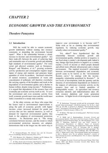
46 Economic Survey of Europe, 2003 No. 2CHART 2.1.1The environmental Kuznets curve: a development-environment relationshipchange towards information-based industries andservices, more efficient technologies, and increaseddemand for environmental quality result in levelling-offand a steady decline of environmental degradation,62 asseen in chart 2.1.1.The issue of whether environmental degradation i)increases monotonically, ii) decreases monotonically,or iii) first increases and then declines along acountry’s development path, has critical implicationsfor policy. A monotonic increase of environmentaldegradation with economic growth calls for strictenvironmental regulations and even limits oneconomic growth to ensure a sustainable scale ofeconomic activity within the ecological life-supportsystem. 63 A monotonic decrease of environmentaldegradation along a country’s development pathsuggests that policies that accelerate economicgrowth lead also to rapid environmentalimprovements and no explicit environmental policiesare needed; indeed, they may be counterproductive ifthey slow down economic growth and thereby delayenvironmental improvement.Finally, if the environmental Kuznets curvehypothesis is supported by evidence, developmentpolicies have the potential of being environmentallybenign over the long run (at high incomes), but theyare also capable of significant environmental damage6263T. Panayotou, Empirical Tests and Policy Analysis , op. cit.K. Arrow, B. Bolin, R. Costanza, P. Dasgupta, C. Folke, C.Holling, B. Jansson, S. Levin, K. Mäler, C. Perings and D. Pimental,“Economic growth, carrying capacity and the environment”, Science, Vol.268, 1995, pp. 520-521.in the short-to-medium run (at low-to-medium-levelincomes). In this case, several issues arise: i) at whatlevel of per capita income is the turning point? ii)How much damage would have taken place, and howcan it be avoided?iii) Would any ecologicalthresholds be violated and irreversible damage takeplace before environmental degradation turns down,and how can they be avoided? iv) Is environmentalimprovement at higher income levels automatic, ordoes it require conscious institutional and policyreforms? And v), how to accelerate the developmentprocess so that developing and transition economiescan attain the same improved economic andenvironmental conditions enjoyed by developedmarket economies?The objective of this paper is to examine theempirical relationship between economic growth andthe environment at different stages of economicdevelopment and explore how economic growthmight be decoupled from environmental pressures.Particular attention is paid to the role of structuralchange, technological change and economic andenvironmental policies in the process of decouplingand the reconciliation of economic and environmentalobjectives. I then examine the experience of the ECEregion in fostering environmentally friendly growth,whether and how it has been possible to decoupleeconomic growth from environmental pressures inthe ECE region. What has been the role of structuralchange, technological change and policy instrumentsin this decoupling for the two major groups ofcountries that constitute the ECE region, thedeveloped market economies and the economies intransition?
Panayotou: Economic Growth and the Environment 472.2 Empirical models of environment andgrowthThe environment-growth debate in the empiricalliterature has centred on the following five questions.First, does the often-hypothesized inverted-U-shapedrelationship between income and environmentaldegradation, known as the environmental Kuznetscurve, actually exist, and if so how robust and generalis it? Second, what is the role of other factors, such aspopulation growth, income distribution, internationaltrade and time-and-space-dependent (rather thanincome-dependent) variables? Third, how relevant is astatistical relationship estimated from cross-country orpanel data to an individual country’s environmentaltrajectory and to the likely path of today’s developingcountries and transition economies. Fourth, what arethe implications of ecological thresholds andirreversible damages for the inverted-U-shapedrelationship between environmental degradation andeconomic growth? Can a static statistical relationshipbe interpreted in terms of carrying capacity, ecosystemresilience and sustainability? Finally, what is the roleof environmental policy both in explaining the shapeof the income-environment relationship, and inlowering the environmental price of economic growthand ensuring more sustainable outcomes?Empirical models of environment and growthconsist usually of reduced form single-equationspecifications relating an environmental impactindicator to a measure of income per capita. Somemodels use emissions of a particular pollutant (e.g.SO2, CO2 or particulates) as dependent variables, whileothers use ambient concentrations of various pollutantsas recorded by monitoring stations; yet other studiesemploy composite indexes of environmentaldegradation. The common independent variable ofmost models is income per capita, but some studies useincome data converted into purchasing power parity(PPP), while others use incomes at market exchangerates. Different studies control for different variables,such as population density, openness to trade, incomedistribution and geographical and institutionalvariables. The functional specification is usuallyquadratic, log quadratic or cubic in income andenvironmental degradation.They are estimatedeconometrically using cross-section or panel data andmany test for country and time-fixed effects. The adhoc specifications and reduced form of these modelsturn them into a “black box” that shrouds theunderlying determinants of environmental quality andcircumscribes their usefulness in policy formulation.There have been some recent efforts to study thetheoretical underpinnings of the environment-incomerelationship and some modest attempts to decomposethe income-environment relationship into itsconstituent scale, composition and abatement effects.However, as Stern64 has concluded, there has been noexplicit empirical testing of the theoretical models andstill we do not have a rigorous and systematicdecomposition analysis.I proceed with an overview of the theoreticalmicrofoundations of the empirical models, followed bya survey of studies whose primary purpose is toestimate the income-environment relationship. I thensurvey attempts at decomposition analysis followed bystudies that focus on mediating or conditioningvariables, such as international trade, as well as onecological and sustainability considerations and issuesof political economy and policy.Finally, I review the experience of the ECEregion in terms of the growth and environmentrelationship and efforts to decouple the two.2.3 Theoretical underpinnings of empiricalmodelsThe characteristics of production and abatementtechnology, and of preferences and their evolutionwith income growth, underlie the shape of the incomeenvironment relationship. Some authors focus onshifts in production technology brought about by thestructural changes accompanying economic growth.65Others have emphasized the characteristics ofabatement technology.66 And yet others have focusedon the properties of preferences and especially theincome elasticity for environmental quality.67 A fewauthors have formulated complete growth models withplausible assumptions about the properties of bothtechnology and preferences from which they deriveenvironmental Kuznets curves (EKCs).68 In thissection, I shall briefly review the main theoreticalstrands of the Kuznets curve literature.64D. Stern, “Progress on the environmental Kuznets curve?”,Environment and Development Economics, Vol. 3, 1998, pp. 173-196.65G. Grossman and A. Kreuger, “Environmental impacts ”, op.cit.; T. Panayotou, Empirical Tests and Policy Analysis , op. cit.66T. Selden and D. Song, op. cit.; J. Andreoni and A. Levinson, TheSimple Analytics of the Environmental Kuznets Curve, NBER WorkingPaper, No. 6739 (Cambridge, MA), September 1998.67K. McConnell, “Income and the demand for environmentalquality”, Environment and Development Economics, Vol. 2, November1997, pp. 383-400; B. Kriström and P. Riera, “Is the income elasticity ofenvironmental improvements less than one?”, Environmental andResource Economics, Vol. 7, Issue 1, pp. 45-55, January 1996; J. Antleand G. Heidebrink, “Environment and development: theory andinternational evidence”, Economic Development and Cultural Change,Vol. 43, April 1995, pp. 603-625.68R. López, “The environment as a factor of production: the effectsof economic growth and trade liberalization”, Journal of EnvironmentalEconomics and Management, Vol. 27, Issue 2, September 1994, pp. 163184; T. Selden and D. Song, op. cit.
48 Economic Survey of Europe, 2003 No. 2The model by López69 consists of two productionsectors, with weak separability between pollution andother factors of production (labour and capital),constant returns to scale and technical change andprices that are exogenously determined.Whenproducers free ride on the environment or pay fixedpollution prices, growth results inescapably in higherpollution levels. When producers pay the full marginalsocial cost of the pollution they generate, the pollutionincome relationship depends on the properties oftechnology and of preferences. With homotheticpreferences pollution levels still increase monotonicallywith income; with non-homothetic preferences, thefaster the marginal utility declines with consumptionlevels and the higher the elasticity of substitutionbetween pollution and other inputs, the less pollutionwill increase with output growth.Empiricallyplausible values for these two parameters result in aninverted-U-shaped relationship between pollution andincome. This tends to explain why in the case ofpollutants such as SO2 and particulates, where thedamage is more evident to consumers and, hence,pollution prices are near their marginal social costs,turning points have been identified at relatively lowincome levels. In contrast, turning points are found atmuch higher income levels, or not at all, for pollutantssuch as CO2, from which damage is less immediateand less evident to consumers, and hence underpriced,if priced at all.Selden and Song,70 using Forster’s71 growth andpollution model with a utility function that is additivelyseparable between consumption and pollution, derive aninverted-U path for pollution and a J-curve forabatement that starts when a given capital stock isachieved; that is, expenditure on pollution abatement iszero until “development has created enoughconsumption and enough environmental damage tomerit expenditures on abatement”.72 Two sets of factorscontribute to an early and rapid increase in abatement:i) on the technology side, large direct effects of growthon pollution and a high marginal effectiveness ofabatement, and ii) on the demand side (preferences),rapidly declining marginal utility of consumption andrapidly rising marginal concern over mountingpollution levels. To the extent that developmentreduces the carrying capacity of the environment, theabatement effort must increase at an increasing rate tooffset the effects of growth on pollution.A number of empirical EKC models haveemphasized the role of the income elasticity of demandfor environmental quality as the theoreticalunderpinning of the inverted-U-shaped relationshipbetween pollution and income.73 Arrow et al.74 statethat because the inverted-U-shaped curve “isconsistent with the notion that people spendproportionately more on environmental quality as theirincome rises, economists have conjectured that thecurve applies to environmental quality generally”. Anumber of earlier studies75 found income elasticitiesfor environmental improvements greater than one.Kriström76 reviewed the evidence from contingentvaluation method (CVM) studies77 that found incomeelasticities for environmental quality much less thanone. Does the finding of a low-income elasticity ofdemand for environmental quality present a problemfor EKC models?McConnell78 examines the role of the incomeelasticity of demand for environmental quality in EKCmodels by adapting a static model of an infinitely livedhousehold in which pollution is generated byconsumption and reduced by abatement. He finds thatthe higher the income elasticity of demand forenvironmental quality, the slower the growth ofpollution when positive, and the faster the declinewhen negative, but there is no special role assigned toincome elasticity equal to or greater than one. In fact,pollution can decline even with a zero or negativeincome elasticity of demand, as when preferences arenon-additive or pollution reduces output (e.g. reducedlabour productivity because of damage to health,material damage due to acid rain or loss of crop outputdue to agricultural externalities). He concludes thatpreferences consistent with a positive income elasticityof demand for environmental quality, while helpful,are neither necessary nor sufficient for an inverted-Ushaped relationship between pollution and income.McConnell found little microeconomic evidence innon-valuation studies that supports a major role for the73W. Beckerman, op. cit.; J. Antle and G. Heidebrink, op. cit.; S.Chaudhuri and A. Pfaff, “Household income, fuel choice and indoor airquality: microfoundations of an environmental Kuznets curve”, ColumbiaUniversity Department of Economics, 1998, mimeo.74T. Boercherding and R. Deacon, “The demand for the services ofnon-federal governments”, American Economic Review, Vol. 62, 1972,pp. 891-901; T. Bergstrom and R. Goodman, “Private demands for publicgoods”, American Economic Review, Vol. 63, No. 3, 1973, pp. 280-296;A. Walters, Noise and Prices (Oxford, Oxford University Press, 1975).69R. López, op. cit.7670T. Seldon and D. Song, op. cit.7771B. Forster, “Optimal capital accumulation in a pollutedenvironment”, The Review of Economic Studies, Vol. 39, 1973, pp. 544547.72T. Selden and D. Song, op. cit., p. 164.K. Arrow et al., op. cit., p. 520.75B. Kriström and P. Riera, op. cit.R. Carson, N. Flores, K. Martin and J. Wright, ContingentValuation and Revealed Preference Methodologies: Comparing theEstimates for Quasi-public Goods, University of California, Departmentof Economics, Discussion Paper No. 94-07 (San Diego), 1994.78K. McConnell, op. cit.
Panayotou: Economic Growth and the Environment 49responsiveness of preferences to income changes inmacroeconomic EKC models.Kriström,79 interpreting the EKC as anequilibrium relationship in which technology andpreference parameters determine its exact shape,proposed a simple model consisting of: a) a utilityfunction of a representative consumer increasing inconsumption and decreasing in pollution; and b) aproduction function with pollution and technologyparameters as inputs. Technological progress isassumed to be exogenous. He interprets the EKC asan expansion path resulting from maximizing welfaresubject to a technology constraint at each point in time;along the optimal path the marginal willingness to payfor environmental quality equals its marginal supplycosts (in terms of forgone output). Along theexpansion path the marginal utility of consumption,which is initially high, declines and the marginaldisutility of pollution (marginal willingness to pay forenvironmental quality) is initially low and rises.Technological progress makes possible moreproduction at each level of environmental quality,which creates both substitution and income effects.The substitution effect is positive for bothconsumption and pollution. The substitution effectdominates at low-income levels and the income effectdominates at high-income levels producing aninverted-U-shaped relationship between pollution andincome. Of course, the exact shape of the relationshipand the turning point, if any, depend on the interplay ofthe technology and preference parameters, which differamong pollutants and circumstances.In overlapping generation models80 pollution isgenerated by consumption activities and is onlypartially internalized as the current generationconsiders the impact of pollution on its own welfarebut not on the welfare of future generations. In thesemodels, the economy is characterized by decliningenvironmental quality when consumption levels arelow, but given sufficient returns to environmentalmaintenance, environmental quality recovers and mayeven improve absolutely with economic growth.Andreoni and Levinson81 derived inverted-Ushaped pollution-income curves from a simple modelwith two commodities, one good and one bad, whichare bundled together. Rising income results inincreased consumption of the good, which generatesmore of the bad. This presents consumers with atrade-off: by sacrificing some consumption of the goodthey can spend some of their income on abatement toreduce the ill effects of the bad. When increasingreturns characterize the abatement technology highincome individuals (or countries) can more easilyachieve more consumption and less pollution thanlow-income individuals (or countries), giving rise to anoptimal pollution-income path that is inverted-Ushaped. The abatement technology is characterized byincreasing returns when it requires lumpy investmentor when the lower marginal cost technology requireslarge fixed costs (e.g. scrubbers or treatment plants);poor economies are not large enough or pollutedenough to obtain a worthwhile return on suchinvestments and end up using low fixed-cost, highmarginal-cost technologies, while rich economies arelarge enough and polluted enough to make effectiveuse of high fixed-cost, low marginal-cost technologies.Different pollutants have different abatementtechnologies and correspondingly the incomeenvironment relationship may or may not be aninverted-U shape. The authors argue that similarresults are obtained from other “good-bad”combinations, e.g. driving a vehicle associated with amortality risk that can be abated by investments insafety equipment: “both the poor who drive very littleand the rich, who invest in safe cars face lower riskfrom driving than middle-income people”. Indeed,empirically, Khan82 found such an inverted-U-shapedrelationship between hydrocarbon emissions andhousehold income in California, and Chaudhuri andPfaff83 between indoor pollution and household incomein Pakistan.In conclusion, while many of the models used ineconometric estimations of the environmental Kuznetscurve have been ad hoc formulations, there has beenno scarcity of theoretical microfoundations of aninverted-U-shape relationship between income andpollution, ranging from production structure, toabatement technology and consumer preferences.2.4 The basic environmental Kuznets curve79B. Kriström, “On a clear day, you might see the environmentalKuznets curve”, Camp Resources (Wilmington, NC), 12-13 August 1999and “Growth, employment and the environment”, Swedish EconomicPolicy Review, 2000, forthcoming.The 1990s saw the advent of the environmentalKuznets curve hypothesis and an explosion of studiesthat tested it for a variety of pollutants. In this section,I review the basic EKC studies that focus on the80A. John and R. Pecchenino, “An overlapping generations model ofgrowth and the environment”, The Economic Journal, Vol. 104, 1994, pp.1393-1410; A. John, R. Pecchenino, D. Schimmelpfennig and S. Schreft,“Short-lived agents and the long-lived environment”, Journal of PublicEconomics, Vol. 58, Issue 1, September 1995, pp. 127-141.81J. Andreoni and A. Levinson, op. cit.82M. Kahn, “A household level environmental Kuznets curve”,Economics Letters, Vol. 59, Issue 2, May 1998, pp. 269-273.83S. Chaudhuri and A. Pfaff, op. cit.
50 Economic Survey of Europe, 2003 No. 2income-environment relationship; in subsequentsections I review studies that focus on mediating orconditioning variables. The annex table summarizes32 empirical studies of the EKC hypothesis and theannex chart depicts these findings in diagrammaticform. The first set of empirical studies appearedindependently in three working papers: by Grossmanand Krueger84 in an NBER working paper as part of astudy of the likely environmental impacts of NAFTA;by Shafik and Bandyopadhyay85 for the World Bank’s1992 World Development Report; and by Panayotou86in a working paper as part of a study for theInternational Labour Office. It is reassuring that theseearly studies found turning points for several pollutants(SO2, NOX and SPM) in a similar income range of 3,000- 5,000 per capita.Grossman and Krueger87 estimated EKCs forSO2, dark matter (smoke) and suspended particlesusing the Global Environmental Monitoring System(GEMS) data for 52 cities in 32 countries during theperiod 1977-1988; per capita GDP data were inpurchasing power parity (PPP) terms. For SO2 anddark matter, they found turning points at 4,000 5,000 per capita; suspended particles continuallydeclined even at low-income levels. However, atincome levels over 10,000- 15,000 all threepollutants began to increase again, a finding whichmay be an artifact of the cubic equation used in theestimation and the limited number of observations athigh-income levels.Shafik and Bandyopadhyay88 estimated EKCs for10 different indicators of environmental degradation,including lack of clean water and sanitation,deforestation, municipal waste, and sulphur oxides andcarbon emissions. Their sample includes observationsfor up to 149 countries during 1960-1990 and theirfunctional specification includes log linear, logquadratic and logarithmic cubic polynomial forms.They found that the lack of clean water and sanitationdeclined uniformly with increasing incomes and overtime; water pollution, municipal waste and carbonemissions increase; and deforestation is independent of84G. Grossman and A. Kreuger, Environmental Impacts of a NorthAmerican Free Trade Agreement, NBER Working Paper, No. 3914(Cambridge, MA), November 1991.85N. Shafik and S. Bandyopadhyay, op. cit.86T. Panayotou, Empirical Tests and Policy Analysis ofEnvironmental Degradation at Different Stages of EconomicDevelopment, ILO Technology and Employment Programme WorkingPaper, WP238 (Geneva), 1993.87G. Grossman and A. Kreuger, “Environmental impacts ”, op. cit.and “Economic growth and the environment”, Quarterly Journal ofEconomics, Vol. 110, Issue 2, May 1995, pp. 353-377.88N. Shafik and S. Bandyopadhyay, op. cit.income levels. In contrast, air pollutants conform tothe EKC hypothesis with turning points at incomelevels between 300 and 4,000. Panayotou, usingcross-section data and a translog specification, foundsimilar results for these pollutants, with turning pointsat income levels ranging from 3,000 to 5,000.89(The lower figures are due to the use of officialexchange rates rather than PPP rates.)Panayotou also found that deforestation alsoconforms to the EKC hypothesis, with a turning pointaround 800 per capita; controlling for income,deforestation is significantly greater in tropical and indensely populated countries. Cropper and Griffiths,90on the other hand, using panel data for 64 countriesover a 30-year period, obtained a turning point fordeforestation in Africa and Latin America between 4,700 and 5,400 (in PPP terms). These turningpoints are a multiple of those found in the Panayotouand Shafik and Bandyopadhyay studies, a possibleconsequence of Cropper and Griffith’s use of paneldata. A study by Antle and Heidebrink,91 which usedcross-section data, found turning points of 1,200(1985 prices) for national parks and 2,000 forafforestation.On the other hand, Bhattari andHammig,92 who used panel data on deforestation for 21countries in Latin America, found an EKC with aturning point of 6,800. Furthermore, earlier studieshave controlled for macroeconomic factors, such as thelevel of indebtedness and for the quality of institutions,which were found to have the expected signs, negativeand positive, respectively.93Returning to urban environmental quality, themid-1990s saw a large number of studies focusing onairborne pollutants. Selden and Song94 estimatedEKCs for SO2, NOX, and SPM and CO usinglongitudinal data on emissions in mostly developedcountries. They found turning points of 8,700 forSO2, 11,200 for NOX, 10,300 for SPM, and 5,600for CO. These are much higher levels than thosefound by Grossman and Krueger, a difference that the89T. Panayotou, Environmental Kuznets Curves , op. cit.;Empirical Tests and Policy Analysis , op. cit.; “Environmentaldegradation at different stages of economic development”, in I. Ahmedand K. Doeleman (eds.), Beyond Rio (The Environmental Crisis andSustainable Livelihoods in the Third World) (Basingstoke, MacMillan,1995).90M. Cropper and C. Griffiths, “The interaction of populationgrowth and environmental quality”, American Economic Review, Vol. 84,1994.91J. Antle and G. Heidebrink, op. cit.92M. Bhattarai and M. Hammig, “An empirical investigation of theenvironmental Kuznets curve for deforestation in Latin America”, paperpresented at the SAEA meeting (Lexington, Kentucky), January 2000.93Ibid.94T. Seldon
CHAPTER 2 ECONOMIC GROWTH AND THE ENVIRONMENT - UNECE . relationship