Transcription
http://excel.fit.vutbr.czDetection of Yoga Poses in Image and VideoJiřı́ KutálekAbstractIn this paper, the concept of a smartphone app detecting Yoga poses and displaying several framesto a user is presented. The goal of this project is proving that even a simple Convolutional NeuralNetwork (CNN) model can be trained to recognize and classify video frames from a Yoga session. Icreated an application in which the videos are manually annotated. The data, consisting of framescaptured from 162 collected videos based on the annotations, is then passed to train a CNN model.The Dataset consists of 22 000 images of 22 different Yoga poses. The frames are captured usingthe OpenCV library, the training process is handled by the TensorFlow platform and the Keras API,and the results are visualized in the TensorBoard toolkit. The Model’s multi-class classificationaccuracy reaches 91% when the binary cross-entropy loss function and the sigmoid activationfunction are used. Despite the experimental results are promising, the main contributions are thedataset forming tools and the Dataset itself, which both helped to confirm the proof-of-concept.Keywords: Yoga Poses Detection — Video Annotation Application — Training CNN for Yoga PosesRecognitionSupplementary Material: Demonstration Video*xkutal09@stud.fit.vutbr.cz, Faculty of Information Technology, Brno University of Technology1. IntroductionOver the last few years, Yoga popularity is rapidlyincreasing. Due to this, there are plenty of instructional videos and Yoga teaching smartphone applications available on the internet. They usually provide adecent workout guide including useful information forpracticing Yoga on one’s own. However, they hardlyever provide a visual workout feedback. This can beobtained either by exercising in front of the mirror, orby recording the session on camera and exploring thevideo. Both might be quite inconvenient.This paper introduces an idea of a smartphone appproviding the workout feedback easily, specifically bychoosing and showing just a few frames, representingthe performed Yoga poses, from the recorded workout session. Thanks to that, a user does not need tomanually seek frames in the video. The main problemobviously is, how does the application know, whichof the many frames in the video to choose and displayto the user? I design a Convolutional Neural Network(CNN) classifying the Yoga images into categoriesbased on the corresponding Yoga poses.In 2016, Convolutional Pose Machines (CPMs) [1]presented an innovative systematic design for how convolutional networks can be incorporated into the posemachine framework [2] for learning image featuresand image-dependent spatial models for the task ofpose estimation. CPM proposed a sequential architecture composed of CNNs that directly operate on beliefmaps from previous stages, producing increasingly refined estimates for part locations, without the need forexplicit graphical model-style inference.
An approach to accurately recognize various Yogaposes using deep learning algorithms [3] has beenpresented in 2019. A hybrid deep learning model isproposed using CNN and LSTM [4] for Yoga recognition on real-time videos, where CNN layer is used toextract features from keypoints of each frame obtainedfrom OpenPose [5] and is followed by LSTM to givetemporal predictions.Unfortunately, these methods are not suitable fora smartphone app as the architecture is too heavy forthe processing units currently in use. Besides that,another paper [6] proposes a system monitoring bodyparts movement and accuracy of different Yoga poses,which aids the user to practice Yoga. However, ituses Microsoft Kinect for human body parts real timedetection, an expensive device most people do not haveat hand.This paper proposes a more practical solution. Allthe user has to do is to record their workout session ona camera and then run the application. After pickingthe input video, several well performed Yoga imagesare selected and displayed on the screen. The greatbenefit is that reviewing a dozen photos is much moreaccessible than watching and rewinding a whole session video. Furthermore, a person is able to eitherevaluate images by their eyes, or save them to galleryand consult with their Yoga instructor later, which mayboth lead to the exercise progression.Up till now, I collected many Yoga videos servingas data resources and created a custom annotation application enabling to form the Dataset from them. Forthis purpose, I wrote a script capturing video framesby the annotations, which forms the Dataset, currentlycontaining tens of thousands of images. Apart formthat, I proposed a CNN model and performed manyexperiments in order to tune it as well as possible.2. BackgroundConvolutional Neural Networks are used for solvingthe image classification problems because of their highaccuracy. The principles behind them, including aninsight into their architecture, are described in thisSection. On top of that, the tools utilized in this workare presented at the end.2.1 Brief Introduction to the CNNsUsing an ordinary Artificial Neural Network (ANN),image classification problems become difficult because2D images need to be converted to one-dimensionalvectors. This increases the number of trainable parameters rapidly, which takes storage and processingcapability. Convolutional Neural Network, a class ofneural networks, convolves the learned features withinput data, and uses 2D convolutional layers, makingthis architecture well suited to processing 2D data,such as images.A CNN typically consists of several convolutionaland pooling layers dealing with feature extraction followed by fully connected layers managing the classification itself (Figure 1). An activation function plays animportant role in feature extraction allowing to classifyeven non-linearly separable data. The complexity ofthe features detected typically grows with the layerdepth.4 feature maps4 pooledfeature maps6 feature maps6 pooledfeature mapsOUTPUTABINPUTCONVOLUTIONALLAYER 1 ReLUPOOLINGLAYER 1CONVOLUTIONALLAYER 2 ReLUPOOLINGLAYER 2FULLY-CONNECTEDLAYER 1Figure 1. Schematic of a Convolutional NeuralNetwork. The feature maps typically graduallydecrease their spatial resolution, while increasing thenumber of channels. Ultimately, the CNN extractsmore and more abstract information and produces adecision with typically very small number of outputs.Convolution is performed on an input image usinga filter or a kernel (small matrix of values), slidingover the image, multiplying its values with the image pixel values and adding them up. The output values are passed through an activation function, addingnon-linearity to a network. A commonly used ReLUfunction zeros the negative values and keeps the positive ones. The convolutional layer outputs are usuallyreferred to as feature maps or channels. Pooling (subsampling) layer then decreases the feature map sizeto reduce the number of computational parameters inthe network. For instance, max pooling, a frequentlyused type of pooling, takes the maximum value in aspecified window. After a few combinations of convolutional and pooling layers, the final output is flattenedand fed into a fully connected layer (a regular ANN)for classification purposes.In 2012, the AlexNet CNN architecture [7] (Fig. 2)dominated the ImageNet ILSVRC challenge [8] andstarted a wave of interest in CNNs as one of the firstmodels stacking convolutional layers directly on topof each other without inserting pooling layers betweenthem. Moreover, it implements the Dropout regularization method [9] to reduce overfitting in the fullyconnected layers.CNNs were starting to get deeper, and the simplestway of improving the deep networks performance is byincreasing their size. Visual Geometry Group (VGG)presented the VGG-16 [10], consisting of 16 weightedlayers and 136 M parameters in total.
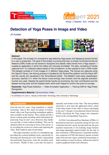
227x227INPUTFiltersFilter sizeCONV2D 96 11x11 ReLUMAX POOLMAX POOLReLU3x3CONV2D 384 3x3FCDROPOUT 50%4096FLATTEN3x3CONV2D 256 5x5Pool sizeReLUFCMAX POOL 3x34096DROPOUT 50%CONV2D 384 3x3ReLUCONV2D 256 3x3ReLUFCUnits1000SoftmaxOUTPUTFigure 2. Schematic of the AlexNet ConvolutionalNeural Network architecture. The model contains fiveconvolutional layers, whose output is passed throughthe ReLU activation function, combined with threemax pooling layers together taking care of featureextraction. During this process, the image resolutionis reduced from 227 227 px to 6 6 px. Then theoutput is flattened and passed to the second part of thenetwork managing the classification by three fullyconnected layers, coupled with two Dropout layersrandomly dropping 50 % of outputs each. The softmaxactivation function is used at the output layer to makepredictions. The network operates with more than a56 M trainable parameters.In 2015, Microsoft Research proposed anothersuccessful model, an extremely deep network calledResNet [11] composed of 152 layers, known for theintroduction of residual blocks.I made few experiments with the AlexNet andVGG-16 CNN models. The results are presented inSection 5.2.2 Work ToolsI capture video screenshots through the OpenCV library [12, 13] and form a dataset from them.The training process itself is in a full control ofthe TensorFlow platform [14, 15] (v2.3 and higher)and its associated deep learning API Keras [16]. I useKeras for dataset loading and configuration, as well asthe CNN model definition and its subsequent training.Thanks to the TensorFlow’s tf.summary moduleI am able to write summary data and visualize themthrough the TensorBoard toolkit1 (Figure 3).All of the scripts are written in the Python2 programming language.3. Forming the DatasetWith the help of my supervisor, I collected 162 Yogavideos containing three different Yoga sequences andbuild a dataset from them. Unfortunately, videos currently come only from two people, which is a too small1 https://github.com/tensorflow/tensorboard2 %80%70%EPOCHS020406080100 120 140Figure 3. Example of the training processvisualization in TensorBoard. This diagram showseight validation accuracy curves, each representing asingle model training process. The x-axis representsthe training epochs, while the y-axis shows theaccuracy. The TensorBoard’s Scalars Dashboardallows a user to visualize many different accuracy orloss curves at once, filter out the unwanted ones,compare the wanted ones and find out additionalinformation about each epoch, such as its duration orthe actual accuracy value. Moreover, the curves areupdated step by step during the training process,making it possible to monitor the training process andreact to changes.sample size to form a truly comprehensive dataset. Butfor now the goal is the proof-of-concept (verifyingthe potential of the idea) and that purpose the Datasetserves well.3.1 Annotating Videos using a Custom Annotation ApplicationThe Dataset for the training itself consists of images,not videos. Therefore, I created an annotation tool(Fig. 4), where the videos are manually annotated. Theannotations define exact frames, at which the trainingand validation frames are being taken.In the video which the application takes on theinput, a person performs one of the predefined Yogasequences, each of them containing several Yoga poses(Figure 5). And each of the poses exercised in theparticular sequence is represented by an annotation.This means that when a pose is done three times duringits corresponding sequence, there is a single annotationfor each of them.The annotations (Figure 6) consist of a pose identifier and five numerical values representing the videoframes defining the time a person is performing thecorresponding Yoga pose. In the app (Figure 4), theframes are marked by the buttons in the bottom leftcorner and the annotations are then displayed in thevideo timeline.
High PlankBEFORESTARTBESTENDAFTERFigure 4. Screenshot of the annotation applicationworkplace. In the top right corner there is a list ofannotations belonging to the currently processedvideo. The annotations are created by the yellowbuttons at the bottom left and visualized by graphs inthe timeline. In addition, the application supportsvideo rewinding and speed changes and providesseveral other features such as video seeking andtimeline zooming.Once done and the progression is saved, a .jsonfile, named by the processed video file, is created.There is a single file for each annotated video storingall of the annotations related. The .json files storingthe annotations are passed to a script randomly takingscreenshots at the specified frames using the OpenCVlibrary, which forms the Dataset.Figure 5. Examples of Yoga poses representing theclasses into which the data is classified.3.2 Data Shape and VolumeDespite the 162 videos come from only two subjectsand the fact that each subject always exercises in asame room, each of the videos is unique. Most of theYoga sessions are recorded by multiple cameras (upto four) positioned in various angles. Furthermore,almost for every session the subjects wear clothes ofdifferent colors and usually change the part of a roomwhere practicing, so that the video background is altered. The light conditions for some sessions vary too,but care should be taken to ensure enough light and notmuch shadow in a footage. Thanks to all these aspectsHigh Plank100150180200300Figure 6. Example of an annotation referring to theHigh Plank Yoga pose. The graph on the rightportrays its corresponding representation in thetimeline. All of the frames between START and ENDsymbolize the time a person is performing the pose,and therefore, the screenshots can be taken during thisperiod. The frame intervals between BEFORE andSTART and between END and AFTER, as well as theBEST frame in each annotation, are not utilized fornow, but could be useful in a future work.the data is quite varied, although the number of peopleproducing the Yoga videos is very low.The Yoga videos are split into two directories separating the training and the validation data by 3 : 1. Thisis done at this early level, because of the potential tomanually choose the source of pictures used for modeltraining (I am able to build both easy and hard datasets).The frame extraction script walks through the directorycontaining the video files iteratively, meaning that allof the classes hold the same amount of data.Currently, I work with the Dataset (Figure 7) containing 44 000 images (2 000 per class/Yoga pose), butthanks to the frame range defined in the annotations, Iam able to create a dataset carrying hundreds of thousands of pictures. The frames are captured with thefixed resolution 256 256 px (squared) and resized ata later stage, when the Dataset is being configured forperformance, into an appropriate shape.However, not all of the 44 000 images are usedfurther in the training process. The frame extractionscript serves only as a giant image collection providerand this collection is updated only when new videosare being integrated into the dataset forming process,which is done occasionally. Moreover, I often alter theDataset size and structure and it takes more than anhour to walk through the videos and capture frames.Therefore, I truly work with 22 000 images randomly chosen from the 44 000 before an every set ofexperiments. As mentioned above, the training andvalidation data is split by 3 : 1, which means that thetraining dataset contains 16 500 images (750 per pose)and the validation dataset consists of 5 500 images(250 per pose).
Figure 7. Samples from the Dataset. The videos aresquare (or trimmed to square if captured otherwise).The subject should be visible during the wholetraining. A defined set of Yoga sequences wasperformed when shooting the videos.4. Training CNN for Yoga Poses RecognitionFigure 8. Augmented image samples. Each of thepictures is taken from a different batch, as all thetransformations applied are same for the images in asingle batch. The augmentation techniques includecolor changes, rotations, flipping, and a central crop.the first training epoch starts (for each epoch there areA complete workflow of how the Dataset is loaded and different transformations applied to the training data).configured, as well as how the actual CNN training Lastly, the prefetch transformation creates an overlapprocess looks like, is described in this Section. As between the data being pre-processed and the modelthe training process is in a full control of the Tensor- execution while training, allowing the later processedFlow platform and the Keras API, a few examples of data to be prepared, while some other data is beingprocessed.functions and utilities used are covered too.During the first training epoch, the loaded pictures4.1 Dataset Loading, Configuration and Arran- are kept in memory (cached) for the subsequent iterations to use them, in order to prevent the DatasetgementIn preparation for model training, the images are loaded becoming a bottleneck during the training process.off disk using the image dataset from directory utility, provided by the tf.keras.preprocessing 4.2 CNN Model Training Processmodule. The Dataset is already divided into training Before the actual training process starts, it is necesdata and validation data, as the videos come from two sary to build the CNN Model. I do this through thedifferent directories. The frame resolution remains at tf.keras.Sequential class grouping a linearthe 256 256 px and the image batch size is usually stack of layers into a single model. The models I exset to 32.periment with consist of six to ten convolutional layersAfter loading, the data is normalized to unify the combined with four or five max pooling layers, foldata distribution of the pixels (the input in the [0, 255] lowed by no more than three fully connected layersrange is rescaled to fit the [0, 1] range) and then resized, (see Figure 9 for an example). I try to design the armostly to 96 96 px, which is the image resolution I chitectures as simple as possible (although the highestmainly operate with.priority is the model efficiency of course). As for theTo fight overfitting in the training process and in- activation functions, I majorly use the Rectified Linearcrease the diversity of the Dataset, I apply various aug- Unit (ReLU) at the hidden layers and switch betweenmentation techniques to the images (Figure 8). These softmax and sigmoid at the output layer.transformations cover picture rotating, horizontal flipFor model evaluation I use the categorical accuping and several image color enhancements, namely racy metric calculating how often predictions matchcontrast, brightness, saturation and hue changes. The one-hot labels, as the data is represented as one-hotcentral region of some pictures is cropped, too. Most Tensors (in one-hot encoding, each class is representedof the techniques are realized using the tf.image by a binary feature – either 1 or 0). Since the labels aremodule. For frame rotations I utilize the tfa.image provided in a one-hot representation, I use the categorone belonging to the TensorFlow Addons repository.ical cross-entropy loss function to compute the crossAll of these techniques are combined together and entropy loss between labels and predictions. However,applied to each image batch of the training data before sometimes I replace it with the binary cross-entropy
224x224INPUTKernels Kernel size Pool sizeCONV2D 32 3x3 ReLUMAX POOLMAX POOLCONV2D 256 3x3ReLUReLUCONV2D 256 3x3ReLUCONV2D 128 3x3ReLUCONV2D 128 3x3CONV2D 128 3x3ReLUMAX POOL2x2CONV2D 64 3x3MAX POOLMAX POOL2x2DROPOUT 20%2x22x22x2ReLUFLATTENDENSE512DENSE128DENSE 22UnitsSigmoidOUTPUTFigure 9. Schematic presenting one of the mostsuccessful CNN models I found during theexperiments. It consists of eight convolutional layers,whose output is passed through the ReLU activationfunction, managing the feature extraction togetherwith five max pooling layers, which consecutivelyreduce the image dimensionality from 224 224 px to7 7 px. Before the final output is flattened and fed tothe first fully connected layer, 20 % of the outputs aredropped (chosen randomly), in order to reduceoverfitting. The Model contains three fully connectedlayers (called Dense in the Keras Sequential API).The sigmoid activation function is used at the outputlayer to make predictions. This Model operates with7, 7 M trainable parameters. Its accuracy is shown inFig. 14.loss function combined with the sigmoid activationfunction at the Model output layer (see Section 5 formore details). On top of that, I use Adam [17] as anoptimizer.The training process happens in epochs. The batchesof training data are fed to the network one-by-one, followed by the validation data batches every epoch. Foreach batch, its samples are used to estimate the errorgradient, which is subsequently used to update themodel weights. At the end of each epoch, the learningrate, specifying how much are the model weights beingupdated, is recalculated.Moreover, I use to visualize images from preferredbatches, in order to both explore the augmented training data and see the correct and wrong label predictionson validation data. During each epoch, right after theModel weights are updated for the last time, scalarTensor values (accuracy and loss) are written to diskusing the tf.summary file writer. By doing so, I amable to visualize these metrics through TensorBoardand track the model training effectively.5. Experimental ResultsI experimented with CNN model architectures (including the AlexNet and VGG-16), data augmentationtechniques and various training parameters such aslearning rate, loss functions or setting the input imagedimensions. Some of them led to interesting findingsor helped to reach great results. In this Section, theexperiments made, as well as the results achieved arepresented.5.1 Findings, Advancements and Model TuningActivation Functions and Loss Functions Perhapsthe most important finding I have made is related toactivation and loss functions. Since I do the multiclass classification, I used to work with the softmaxactivation function, normalizing the network outputto a probability distribution over predicted classes, together with the categorical cross-entropy loss function.But, after a consultation with my supervisor, I foundout that a combination of the sigmoid activation function and the binary cross-entropy loss function is moreefficient.This finding was confirmed across many CNNmodels, where all the networks implementing the sigmoid function had about 4 % higher validation accuracy, than the models using the softmax. From thatmoment, most of the models tested use the sigmoid activation function at the output layer instead of softmax.Model Architectures I experimented with more thana hundred CNN models so far. Firstly, I tested the partof a CNN model dealing with feature extraction (convolutional and max pooling layers). Working with the96 96 px image resolution, I found out that the Modelshould contain at least four consecutive combinationsof convolutional and pooling layers to make decentpredictions. Besides, I ascertained that a too low number of convolutional filters leads to worse validationaccuracy and more unstable results (an example of thiskind of model is shown in Fig. 10).96x96INPUTKernels Kernel size Pool sizeCONV2D 83x3 ReLUMAX POOLMAX POOL2x2CONV2D 64 3x3 ReLUCONV2D 16 3x3MAX POOLReLUCONV2D 32 3x3CONV2D 64 3x3MAX POOL2x2ReLUDROPOUT 20%2x2DENSE2x2CONV2D 32 3x3FLATTENReLUReLUDENSE 22Units64SoftmaxOUTPUTFigure 10. Schematic of a lightweight CNN modelarchitecture. The low number of convolutionalfilters/kernels leads to very low number of trainableparameters in the network (only 200 000). However,this fact causes about 10 % worse model accuracycompared to a similar model with more filters, andmore unstable results, as the validation accuracy curvevery fluctuates each training epoch. Therefore, usingsuch a low number of kernels may be inappropriate.
After that, I experimented with the number of fullyconnected layers and their units. Unfortunately, theoutcomes were all quite similar to each other (the bestones did not stand out much), meaning that this testingbrought out hardly thrilling results. I only found outthat two or three dense layers might be a reasonablenumber.Apart from all those relatively basic models, AlexNet(Fig. 2) and VGG-16, which far outweigh the others by complexity and number of training parameters,were tested too. The VGG-16 model structure turnedout to be probably too complicated for my unvarieddata, as the network was not able to learn anything.The AlexNet, having about 80 M parameters less thanVGG-16, showed itself in a better light as the validation accuracy reaches up to 80 % (see Figure 11).Nevertheless, these results are still worse than the bestones achieved by the simpler models (as seen in Figure 14).TRAINING ACCURACYof the techniques separately, and then I combined themtogether. For instance, I found out that the best resultsare achieved when rotating the image by 10 to 20 degrees in both directions, or when the brightness of apicture is changed just minimally. Another experimental results (presented in Fig. 12) showed how muchshould be the image cropped in the central region.VALIDATION ACCURACYCATEGORICALCROSSENTROPY SOFTMAXCATEGORICALCROSSENTROPY SOFTMAXBINARYCROSSENTROPY SIGMOIDBINARYCROSSENTROPY SIGMOIDFigure 11. Visualization of the experiments madewith the AlexNet CNN model. Each diagram groupsresults of a few measurements together. Thehorizontal axis represents training epochs, while thevertical axis represents training or validation accuracy.The AlexNet originally uses the softmax activationfunction at the output layer, but the sigmoid(combined with an appropriate cross-entropy lossfunction) was tested out of curiosity too. The modelusing the sigmoid variant reaches slightly betterresults. It is clear to see that the network is trainedperfectly in just about 50 epochs, but the validationaccuracy does not exceed 80 %. Apparently, it doesnot generalize well at all.Data Augmentation Techniques Data augmenta-tion proved itself to be very useful in fighting the modeloverfitting. Due to this, I widely experimented withall the individual transformation techniques (rotations,color changes and cropping), in order to set their parameters as precisely as possible. Firstly, I tested eachFigure 12. A heatmap visualizing the results of anexperiment with the central crop data augmentationtechnique. An image is cropped in its central regionwith a given probability. The individual heatmapvalues represent the average validation accuracy in thelast 40 epochs of the model. The values on the verticalaxis represent the chance of cropping all images in abatch, while the horizontal axis represents the valuesof how much are the images being cropped (1.0 standsfor no crop, while 0.5 means that the outer half of animage in cropped out). The heatmap shows thatleaving about 70% of the original image (cropping out30% of the outer region) brings out the best results.Besides, it is clear to see that the crop probability doesnot affect the results much.The latest experiments doneso far analyze which of the Yoga poses sees the network as similar to each other. A custom confusionmatrix, showing only the wrong decision for each pose,was designed for this purpose (see it in Figure 13). Theresults show that all the three “Warrior III.” Yogaposes are often misclassified by each other. A similartrend can be observed by the “Thunderbolt.” poses.Both of the High Plank and Low Cobra are quite often classified as the Four Limbed Staff pose. Besides,the two “Warrior I.” Yoga poses seem interesting asthey are quite often classified as each other, but hardlyever classified as the other poses.Yoga Poses Similarity
three dense layers (Fig. 9), reached the 100 % trainingaccuracy in a few tens of epochs, and demonstrated itscapability to detect Yoga poses by achieving the 91 %validation accuracy (as shown in Figure 14).However, the 91 % were achieved using a “hard”dataset, into which videos were selected precisely inorder to make the model predictions as hard as possible. When testing the Model on an “easy” validationdataset, into which videos were chosen to be similarto the videos chosen to form the training dataset, thevalidation accuracy reached 95 %.But, it is fair to say that the Model is able to detectYoga poses with the 91 % accuracy when trained onthis particular Dataset, because the results reachedwith the “easy” datasets may probably not be valid.Figure 13. A confusion matrix, but is shows only thewrong decisions for each Yoga pose. Each valuerepresents the number of how many times has a posebeen misclassified by another one (the horizontal axisshows the predicted labels and the vertical axis showsthe true labels). The aim of this visualization is onlyto show the possible similarity of the poses, not tomeasure how well are the poses being detected by amodel. The results show that all the three “WarriorIII.” poses are quite similar to each other and thesame holds for the “Thunderbold.” ones. HighPlank and Low Cobra are often classified as FourLimbed Staff, while the two “Warrior I.” posesare similar to each other, but unlike the others.I experimented with the learning ratetoo. I originally used constant values for every epoch(approximately in the range of 2 10 4 to 7 10 3 ),but then I started operating with several partly custombuilt algorithms updating the learning rate dynamicallyat the end of each epoch. Nearly all of these broughtbetter results compared to the measurements madewith the static values. The learning rate is one of themost important model hyperparameters, but finding itsoptimal values is a difficult task.Learning Rate5.2 Achieved ResultsFor most of the experiments, the frames were resizedto the 96 96 px, which is expected as a good compromise providing a decent image resolution and areasonab
based on the corresponding Yoga poses. In 2016, Convolutional Pose Machines (CPMs) [1] presented an innovative systematic design for how con-volutional networks can be incorporated into the pose machine framework [2] for learning image features and image-dependent spatial models for the task of pose estimation. CPM proposed a sequential architec-