Transcription
This is a postprint of J. Chem. Theory Comput., 2015, 11, pp 4220–4225 Theoriginal article can be found 5b00601A comprehensive comparison of the IEFPCM and SS(V)PEcontinuum solvation methods with the COSMO approachA. Klamt1,2, C. Moya3 and J. Palomar312COSMOlogic GmbH&CoKG, Imbacher Weg 46, D-51379 Leverkusen, GermanyInstitute of Physical and Theoretical Chemistry, Universität Regensburg, Germany3Sección de Ingeniería Química. Universidad Autónoma de Madrid, Madrid, Spain* e-mail: klamt@cosmologic.deAbstractDielectric continuum models are popular for modeling solvent effects in quantumchemical calculations. The polarizable continuum model (PCM) was originallypublished exploiting the exact dielectric boundary condition. This is nowadays calledDPCM. The conductor-like screening model (COSMO) introduced a simplified andslightly empirical scaled conductor boundary condition, which turned out to reducethe errors resulting from outlying charge. This was implemented in PCM as CPCM.Later the integral equation formalism (IEFPCM) and the formally identical SS(V)PEmodel of Chipman introduced a modified dielectric boundary condition combiningthe dielectric exactness of DPCM with the reduced outlying charge sensitivity ofCOSMO. In this paper we demonstrate on two huge datasets of neutral and ionicsolutes that no significant difference can be observed between the COSMO andIEFPCM, if the correct scaling factor is chosen for COSMO.IntroductionThe dielectric continuum approach is the most widely used class of methods formodeling solvent effects in quantum chemical calculations and the apparent surfacecharge (ASC) models comprise the most popular subclass of these.1 Its firstrepresentative is the polarizable continuum model (PCM)2, which was originallypublished using the exact dielectric boundary condition (EDBC) for the calculation ofthe vector of polarization charge densities on the surface segments of the solutecavity . Later this original version got named DPCM. In 1993 Klamt and
Schüürmann presented the completely independently derived conductor-likescreening model (COSMO)3, which makes use of the much simpler boundarycondition of a conductor and takes into account the reduction of the polarizationcharge densities occurring at finite permittivity by a slightly empirical scaling xf ( ) 1 x(1)where x was argued to be optimally chosen as 0.5 for neutral solutes, while for ions x 0 should be the best choice. Theoretically COSMO is exact in the limit of ,but the finite behavior is slightly approximate. A big advantage of COSMO over theEDBC was the fact that it only requires the solute electrostatic potential X on thecavity of solute X, while the EDBC requires the normal component of the soluteelectric field EXn , which is much more complicated to calculate and more sensitive tonumerical noise. But the main advantage was only detected later: COSMO suffersmuch less from outlying charge errors (OCE)4 than solvation models using the EDBC,because X is an order of magnitude less influenced than EXn by the fact, that incontinuum solvation models almost inevitably some small part of the total electrondensity of the solute is located outside the solute cavity, while the dielectriccontinuum approach assumes to find all solute charge inside the cavity. Theseadvantages of the COSMO method motivated Barone and Cossi to implement theCOSMO boundary condition within the PCM framework, resulting in the so-calledCPCM model5. Unfortunately the default value for x in the COSMO scaling functionwas set to zero in CPCM, and not to 0.5 as in the original COSMO. Cossi et al. latershowed that the agreement of the results of DPCM and CPCM improves, if for neutralcompounds a value of x 0.5 is chosen, i.e. they confirmed that the original COSMOchoice of x is preferable.6 But the official releases of CPCM in the Gaussian program7do not allow the user to set this value. Hence CPCM is most often used with anunfavorable scaling function.In 1997 Chipman8 started to develop a number of alternative boundary conditions forASC continuum solvation models with the special focus of taking into account thevolume polarization caused by the charge density outside the cavity. As thecomputationally most practical result he derived the SS(V)PE model, in which the (V)denotes approximate volume polarization. As COSMO, this model does only require
the electrostatic potential vector X on the cavity and avoids using the electrostaticfield normal components EXn . At the costs of being numerically more expensive thanCOSMO, it does not require any empirically adjusted parameter beyond the cavitydefinition itself, which is empirical in all CSMs.In 1997 Cances et al.9 published a new and rather general framework for ASCcontinuum solvation models, the so-called integral equation formalism IEF, whicheven allowed for the description of anisotropic dielectric continua. A year later asimplified and computationally much more efficient version of the IEF was presentedby Mennucci et al.,10 which was now again restricted to isotropic solvents, butavoided the use of the problematic EXn . Later it turned out that this method, which isnowadays used under the name IEFPCM, is identical with Chipman’s SS(V)PE, asproven in the excellent theoretical comparison of the different ASC solvation modelsby Chipman. A third, COSMO-based derivation of the same equation was proposedby Klamt while studying the original IEFPCM publication in 1997. This derivation,which was published in Chipman’s paper, elucidates the close similarity betweenCOSMO and SS(V)PE/IEFPCM11.Summarizing the situation, the SS(V)PE/IEFPCM equation has been independentlyderived by three groups and is currently considered as the best available boundarycondition for ASC isotropic dielectric continuum solvation models, combining arobustness with respect to outlying charge effects and computational efficiency. Fromthe theoretical equations it is obvious that in the limit of SS(V)PE/IEFPCMmust be identical to the older COSMO model, which is the algorithmically simplestand computationally least demanding of all ASC models. For finite values of COSMO is slightly more empirical. But it is not known, how big the deviations ofCOSMO and SS(V)PE/IEFPCM are in practice and whether the additionalcomplexity of SS(V)PE/IEFPCM is really warranted by more accurate results.Therefore, in this paper we investigate systematically the practical differences ofCOSMO and SS(V)PE/IEFPCM solvation models.Theory
Using the notations introduced in the COSMO paper, the three methods consideredhere can be described as follows. Let us start with a solute X and a closed cavity defining the boundary of the dielectric continuum of strength embedding X. Let be represented by m sufficiently small surface segments. Let be the vector of the mpolarization charge densities on the segments and S shall be a diagonal matrix of them segment areas. Let A be the symmetric Coulomb interaction matrix of the chargeson the segments, with diagonal elements representing the self-interactions. Let X bethe vector of the solute electrostatic potential on the m segments, and EXn thecorresponding vector of the electrostatic field normal components. Then the exactdielectric boundary condition used in DPCM reads4 1 XE n D S 1 (2)where D is the non-symmetric matrix generating the electric field normal vectorsresulting from the polarization charges on the m segments. The COSMO boundarycondition reads0 1 X AS x(3)For this simply is the grounded conductor boundary condition of vanishing totalpotential on the conductor surface.As mentioned above, the SS(V)PE/IEFPCM boundary condition can be easily derivedfrom a combination of the EDBC and the COSMO boundary condition. If weintroduce * as the polarization charge densities produced in the limit of infinite and if we make use of the fact that under the assumption of all solute charge beinginside the cavity the polarization charges arising from the conductor boundarycondition must be identical with those resulting from the EDBC, then we getE n 4 I D S *X(4)and * A 1 S 1 X(5)Inserting eq. 5 into eq. 4 we get E n 4 I D S A S D 4 SX 1 1X 1 A 1 X(6)
Now we can use this expression for replacing the problematic electric field normalvector EXn in the EDBC, i.e. in eq. 2, yielding4 1 1 1 1XD 4 S A D S 1 1(7)which after short reorganization yields the SS(V)PE/IEFPCM boundary condition 1 1 1 1X 4 I 1 D S 1 D 4 S A (8)This derivation clearly shows that the more favorable behavior of SS(V)PE/IEFPCMcompared to the EDBC and thus DPCM, which sometimes is argued to result fromtaking into account volume polarization, just arises from replacing the problematicelectric field normal vector EXn based on a COSMO expression. It also shows thatSS(V)PE/IEFPCM is algorithmically much more complicated and expensive andmore sensitive to numerical noise than COSMO, because it requires the nonsymmetric D-matrix of the normal electric field components generated by thescreening charges in addition to the symmetric COSMO matrix A.MethodsFor a comparison of the different ASC boundary conditions it is required to use anotherwise identical implementation of the dielectric continuum solvation methods in aquantum chemical package, because any differences in the cavity construction caneasily cause much larger deviations than those arising from different choices of theboundary conditions. For that reason we have chosen the Gaussian09 software whichoffers DPCM, CPCM and IEFPCM as options. Since SS(V)PE and IEFPCM areidentical and since IEFPCM is the name of the method in Gaussian097, we will denotethe SS(V)PE/IEFPCM method shortly as IEFPCM further on. Unfortunately there isno explicit keyword to change the x-parameter in the COSMO scaling function, whichis set to zero in Gaussian09. Nevertheless, this lack can be easily overcome by usingan effective value ( x) of the dielectric permittivity , which results in the samevalue of the scaling function as if a special value of x would have been used. It isdefined by: ( , x) 1 1 ( , x) xand thus yields(9)
( , x) xx 1(10)In this way we considered three variants of CPCM, one corresponding to theGaussian09 default (CPCM with x 0), one corresponding to the x 0.5, as suggestedin the original COSMO implementation, and one with an optimized value of x inorder to achieve optimal agreement with IEFPCM.In addition to the variation of the methods and x-parameter we modified the radiiscaling parameter in 0.1 steps from 0.9 to 1.3. The default value is 1.1. By choosingthe smaller radii we could study the behavior of the different methods in the limit oflarge amounts of outlying charge, and with the large radii the amount of outlyingcharge is reduced to very small amounts.All quantum calculations have been performed using the density functional theoryusing the BVP86/TZVP/DGA1 computational level.12-14All dielectric solvation energies are reported as differences between total energies invacuum and in the dielectric continuum, employing the different dielectric continuummodels.Data setsIn order to perform a rigorous comparison we looked for representative and unbiasedset of compounds to be considered in the study. We decided to consider the 318neutral solutes in the SM8 solvation free energy data set15, which has been consideredin other comparisons of solvation models before.16 This choice should guarantee thatall major compounds classes, for which experimental solvation data are available, arerepresented. The geometries were taken from the BP-TZVP gas phase geometryoptimizations recently published in a study on the D-COSMO-RS solvation model.17For the ions we selected a set of 20 diverse anions and 20 diverse cations from theCOSMObaseIL database for ionic liquids18.
The coordinates for all 358 compounds are given in the Supporting Information.The differences between the dielectric solvation energy obtained by the continuummodels were quantified by calculating the root mean square deviation (RMSD) usingIEFPCM as reference: (𝐸 𝐸𝐼𝐸𝐹𝑃𝐶𝑀 )2𝑅𝑀𝑆𝐷 𝑛(11)ResultsNeutral solutesFor all 318 neutral solutes first the vacuum energy was calculated. Then dielectriccontinuum solvation models were performed for 50 different parameter combinations:1) dielectric permittivity 2 and (represented as 9999)2) radii scaling factor :0.9, 1.0, 1.1, 1.2, 1.33) CSM variant:IEFPCM, DPCM, CPCM (x 0.0,0.5,0.45, 0.37, 0.43)Thus in total 51*318 16218 quantum calculations have been performed for theneutral compounds. All results are reported in table SI1, except for CPCM with x 0.37 and 0.43, which are considered as intermediate results for finding the optimal xvalue of 0.45. Table 1 shows the statistical measures for all calculations for neutrals.
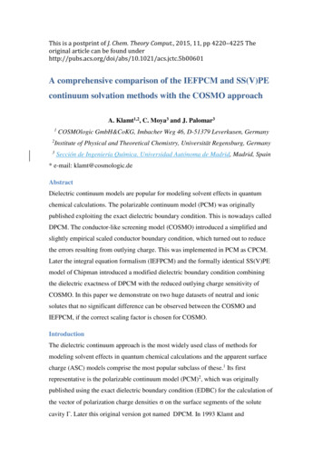
Solvation Energy (kcal/mol) α 0.9 ; ε 28166124CPCM x 0.5CPCM x 0.45CPCM x 0DPCM2Solvation Energy (kcal/mol) α 0.9 ; ε 16Figure 1: a) Dielectric solvation energies for DPCM, CPCM(x 0, 0.5, 0.45) for 318neutral compounds at dielectric permittivity of 2. b) Same differences for dielectricpermittivity . Only one CPCM line is plotted, because the different x values yieldidentical results in this limit. All data points are plotted vs. the IEFPCM result.r2RMSD (kcal/mol)IEFPCMε 2IEFPCMε CPCMx 0.50CPCMx 0.45CPCMx 00.911.11.21.30.911.11.21.30.151 0.107 0.078 0.059 0.045 0.992 0.993 0.993 0.993 0.9930.130 0.094 0.071 0.056 0.044 0.992 0.993 0.993 0.993 0.9930.660 0.484 0.373 0.294 0.235 0.993 0.993 0.993 0.993 0.994DPCM0.505 0.212 0.118 0.061 0.030 0.914 0.960 0.982 0.992 0.997CPCM0.000 0.000 0.000 0.000 0.000 1.000 1.000 1.000 1.000 1.000DPCM1.268 0.758 0.419 0.210 0.103 0.894 0.945 0.976 0.990 0.996Table 1: Statistical measures for the comparison of dielectric solvation energy of neutralcompounds obtained by CPCM and DPCM to those by IEFPCM.Figure 1 shows the results for the default cavity size ( 1.1) and dielectricpermittivity of 2 and , respectively. Table 1 shows the statistical measures for all20
calculations for neutrals, except for CPCM with x 0.37 and 0.43, which areconsidered as intermediate results for finding the optimal x-value of 0.45.Astheoretically expected, in the limit of a perfect agreement of CPCM andIEFPCM is achieved. DPCM shows substantial deviations resulting from the outlyingcharge problem. The largest deviation of DPCM arises for methyl 3-methyl-4thiomethoxyphenylthiophosphate, for which DPCM underestimates the screeningenergy by more than 25%. At the lower limit of solvent dielectric constants, i.e. for 2, CPCM with x 0, i.e. the default CPCM in Gaussian, overestimates the dielectricsolvation energies systematically, resulting in a RMSD of 0.37 kcal/mol, but with anexcellent correlation of r² 0.993, while CPCM with the original COSMO default x 0.5, yields the same excellent correlation, but a RMSD of only 0.073 kcal/mol. Thebest agreement between IEFPCM and CPCM can be achieved using x 0.45,reducing the RMSD to 0.071 kcal/mol. Nevertheless, we do not consider this smallincrease to be relevant. We thus propose to stay with x 0.5 for neutral solutes.
Solvation Energy (kcal/mol) α 0.9 ; ε 28166124CPCM x 0.5CPCM x 0.45CPCM x 0DPCM2Solvation Energy (kcal/mol) α 0.9 ; ε 1620Figure 2: Same data as shown in figure 1, but here for smaller cavity radii, i.e. 0.9Solvation Energy (kcal/mol) α 1.3; ε 2486OTHEROTHER3Solvation Energy (kcal/mol) α 1.3; ε 2CPCM x 0.5CPCM x 0.45CPCM x 0DPCM142CPCMDPCM00012IEFPCM34024IEFPCM6Figure 3: Same data as shown in figure 1, but here for larger cavity radii, i.e. 1.3Figures 2 and 3 show the same plots as Figure 1, but now at reduced cavity radii ( 0.9) and increased cavity radii ( 1.3). At reduced cavity radii all solvation energiesare increased, and the amount of outlying charge is much larger than for 1.1. Forthe larger cavities, i.e. 1.3, the deviations and the correlation between DPCM and8
IEFPCM strongly increase at both 2 and . But the effect of the outlyingcharge on the CPCM and IEFPCM is nearly identical. At there still is nodifference, and at 2 the correlation coefficients between all CPCM variants andIEFPCM stay the same as they were at 1.1. They also stay unchanged for 1.3.As clearly visible in Figure 3, DPCM converges against IEFPCM in the limit ofalmost vanishing outlying charge.Ionic solutesFor the 40 ions again 2 and are considered, but for CPCM only x 0 isconsidered, since this is the default of CPCM and it agrees with the x-value for ionssuggested in the original COSMO publication. As for the neutral solutes five valuesof the radii scaling factor are considered.Figure 4: Dielectric solvation energies for 40 ions for (a) default radii with 1.1 andSolvation Energy (kcal/mol) α 0.9Solvation Energy (kcal/mol) α 1.1125125100OTHEROTHER1007550CPCM ε 2DPCM ε 2CPCM ε DPCM ε 2500255075100IEFPCM(b) reduced cavity radii with 0.9.125RMSD (kcal/mole)7550CPCM ε 2DPCM ε 2CPCM ε DPCM ε 2500255075IEFPCMr2100125
IEFPCMε 2IEFPCMε 0.2890.1470.0470.7090.937Table 2: Statistical measures for the comparison of dielectric solvation energy of ionicsolutes obtained by CPCM and DPCM to those by IEFPCM.Figure 4 shows the dielectric solvation energies of all ions calculated with CPCM(x 0) and DPCM at 2 and , plotted versus the respective IEFPCM results.The statistics of all ion results is given in Table 2. Again a perfect agreement ofCPCM and IEFPCM is achieved at , and with a correlation coefficient of r² 0.993 an almost perfect agreement of the two methods is also achieved at 2.DPCM again suffers dramatically from the outlying charge effect. The correlationcoefficient of the DPCM results vs. the IEFPCM results is as low as r² 0.047 at bothvalues of All dielectric solvation energies for anions are underestimated by DPCM,because the complete neglect of the outlying electron density reduces the effectivecharge of anions. The opposite happens for cations. For the reduced cavity radii theoutlying charge errors of DPCM become so large that even an inverse correlation withIEFPCM occurs.Zwitterionic solutesAfter finishing our project the interesting question was raised which choice of the xparameter should be used for neutral and charged zwitterions, respectively. Thereforewe added a small study on 4 neutral zwitterionic aminoacids and two chargedzwitterions. For all of them we performed calculations with IEFPCM and CPCM withx 0.5 and x 1. The results are shown in Figure 5 and detailed data are given in tableSI1. When using the default value of x according the overall charge of the solute, i.e.x 0.5 for the neutral zwitterions and x 0 for the ionic zwitterions, a correlationcoefficient of r² 0.9977 is achieved between the CPCM and IEFPCM results.Forcing the regression line to zero offset still leaves an excellent correlation of
r² 0.988. Therefore it appears that the choice of x should be made according to theoverall charge of the solute even for zwitterions.50X 0X 0.540x def30CPCMy 1.12x - 2.4R² 0.99772010001020304050IEFPCMFigure 5: Dielectric solvation energies (kcal/mol) for 4 neutral and 2 chargedzwitterions. The data for glutamine and glycine are indistinguishably close.ConclusionsThe integral equation formalism in its second version, as implemented in Gaussian09,and the formally identical SS(V)PE formalism are widely accepted as the currently bestcompromise between theoretical exactness and computational efficiency for dielectricsolvation models. Nevertheless, almost identical dielectric solvation energies can beachieved by the simpler COSMO method when using the originally proposed dielectricscaling factor with the empirical parameter x 0.5 for neutral solutes and x 0 for ions.With this choice of x, COSMO is essentially as good as IEFPCM/ SS(V)PE not only inhighly dielectric solvents, but also in non-polar solvents. Furthermore, the generalidentity of IEFPCM/ SS(V)PE and COSMO in the limit of and the excellentagreement of COSMO and IEFPCM/ SS(V)PE at 2 even at large amounts ofoutlying charge disproof the assumption that SS(V)PE (and thus IEFPCM) would inany way be better in taking into account the outlying charge effects by some kind ofapproximate volume polarization term. The huge advantage of these methods over theclassical DPCM just results from the elimination of the problematic normal electric
field component from the boundary condition by making use of the conductor limitwhich was avoided from the beginning in COSMO model.All other parameters of continuum solvation methods, e.g. the choice of theconstruction method and radii for the cavities, the choice of the quantum chemicalmethod and basis set, and the non-electrostatic contributions will have a much largerinfluence on the quality of continuum solvation calculations than the choice of thetheoretically slightly better justified IEFPCM/ SS(V)PE. Considering the facts that theentire dielectric continuum solvation concept is only a crude approximation to thesituation in real solvents19 , and that the currently best overall agreement betweencalculated and experimental solvation free energies is in the order of 0.5 – 1 kcal/mol(RMSD)16,17, the small theoretical accuracy gain of 0.07 kcal/mol (RMSD) ofIEFPCM/ SS(V)PE vs. COSMO found in our benchmark lets the justification for theconsiderable additional algorithmic and computational expenses of the advancedmethods appear questionable.Supporting informationThe supporting information contains the names and geometries in xyz format of allused solutes in the dataset. Furthermore, all calculated total energies are reported inTable SI1.
13)(14)(15)Tomasi, J.; Mennucci, B.; Cammi, R. Quantum Mechanical ContinuumSolvation Models. Chem. Rev. 2005, 105, 2999–3094.Miertuš, S.; Scrocco, E.; Tomasi, J. Electrostatic Interaction of a Solute with aContinuum. A Direct Utilizaion of AB Initio Molecular Potentials for thePrevision of Solvent Effects. Chem. Phys. 1981, 55, 117–129.Klamt, A.; Schüürmann, G. COSMO: A New Approach to Dielectric Screeningin Solvents with Explicit Expressions for the Screening Energy and ItsGradient. J. Chem. Soc. Perkin Trans. 2 1993, 1993, 799–805.Klamt, A.; Jonas, V. Treatment of the Outlying Charge in Continuum SolvationModels. J. Chem. Phys. 1996, 105, 9972.Barone, V.; Cossi, M. Quantum Calculation of Molecular Energies and EnergyGradients in Solution by a Conductor Solvent Model. J. Phys. Chem. A 1998,102, 1995–2001.Cossi, M.; Rega, N.; Scalmani, G.; Barone, V. Energies, Structures, andElectronic Properties of Molecules in Solution with the C-PCM SolvationModel. J. Comput. Chem. 2003, 24, 669–681.Frisch, M. J.; Trucks, G. W.; Schlegel, H. B.; Scuseria, G. E.; Robb, M. A.;Cheeseman, J. R.; Scalmani, G.; Barone, V.; Mennucci, B.; Petersson, G. A.;Nakatsuji, H.; Caricato, M.; Li, X.; Hratchian, H. P.; Izmaylov, A.; Bloino, J.;Zheng, G.; Sonnenberg, J. L.; Hada, M.; Ehara, M.; Toyota, K.; Fukuda, R.;Hasegawa, J.; Ishida, M.; Nakajima, T.; Honda, Y.; Kitao, O.; Nakai, H.;Vreven, T.; Montgomery, Jr., J. A.; Peralta, J. E.; Ogliaro, F.; Bearpark, M.;Heyd, J. J. Gaussian 09, Revision D.01; Gaussian Inc.: Wallingfort, CT, USA,2009.Chipman, D. M. Charge Penetration in Dielectric Models of Solvation. J.Chem. Phys. 1997, 106, 10194.Cancès, E.; Mennucci, B.; Tomasi, J. A New Integral Equation Formalism forthe Polarizable Continuum Model: Theoretical Background and Applications toIsotropic and Anisotropic Dielectrics. J. Chem. Phys. 1997, 107, 3032.Mennucci, B.; Cammi, R.; Tomasi, J. Excited States and Solvatochromic Shiftswithin a Nonequilibrium Solvation Approach: A New Formulation of theIntegral Equation Formalism Method at the Self-Consistent Field,Configuration Interaction, and Multiconfiguration Self-Consistent Field Level.J. Chem. Phys. 1998, 109, 2798.Chipman, D. M. Comparison of Solvent Reaction Field Representations. Theor.Chem. Acc. 2002, 107, 80–89.Perdew, J. P. Density-Functional Approximation for the Correlation Energy ofthe Inhomogeneous Electron Gas. Phys. Rev. B 1986, 33, 8822–8824.Sosa, C.; Andzelm, J.; Elkin, B. C.; Wimmer, E.; Dobbs, K. D.; Dixon, D. A. ALocal Density Functional Study of the Structure and Vibrational Frequencies ofMolecular Transition-Metal Compounds. J. Phys. Chem. 1992, 96 (16), 6630–6636.Schäfer, A.; Huber, C.; Ahlrichs, R. Fully Optimized Contracted GaussianBasis Sets of Triple Zeta Valence Quality for Atoms Li to Kr. J. Chem. Phys.1994, 100, 5829.Marenich, A. V.; Olson, R. M.; Kelly, C. P.; Cramer, C. J.; Truhlar, D. G. SelfConsistent Reaction Field Model for Aqueous and Nonaqueous SolutionsBased on Accurate Polarized Partial Charges. J. Chem. Theory Comput. 2007,3, 2011–2033.
(16) Klamt, A.; Mennucci, B.; Tomasi, J.; Barone, V.; Curutchet, C.; Orozco, M.;Luque, F. J. On the Performance of Continuum Solvation Methods. AComment on “Universal Approaches to Solvation Modeling.” Acc. Chem. Res.2009, 42, 489–492.(17) Klamt, A.; Diedenhofen, M. Calculation of Solvation Free Energies withDCOSMO-RS. J. Phys. Chem. A 2015, 119, 5439–5445.(18) COSMObaseIL; COSMOlogic GmbH & Co. KG; http://www.cosmologic.de(01 June 2015) Leverkusen, Germany, 2014.(19) Klamt, A. COSMO-RS From Quantum Chemistry to Fluid PhaseThermodynamics and Drug Design; Elsevier: Amsterdam, The Netherlands;Boston, MA, USA, 2005, pp 30-32
TOC graphics:
CPCM model5. Unfortunately the default value for x in the COSMO scaling function was set to zero in CPCM, and not to 0.5 as in the original COSMO. Cossi et al. later showed that the agreement of the results of DPCM and CPCM improves, if for neutral compounds a value of x 0.5 is chosen, i.e. they confirmed that the original COSMO