Transcription
Tutorials in Quantitative Methods for Psychology2006, Vol. 2(1), p. 26‐37.Collecting and analyzing data in multidimensional scalingexperiments: A guide for psychologists using SPSSGyslain GiguèreUniversité du Québec à MontréalThis paper aims at providing a quick and simple guide to using a multidimensional scalingprocedure to analyze experimental data. First, the operations of data collection and preparationare described. Next, instructions for data analysis using the ALSCAL procedure (Takane, Young& DeLeeuw, 1977), found in SPSS, are detailed. Overall, a description of useful commands,measures and graphs is provided. Emphasis is made on experimental designs and program use,rather than the description of techniques in an algebraic or geometrical fashion.In science, being able synthesize data using a smallernumber of descriptors constitutes the first step tounderstanding. Hence, when one must extract usefulinformation from a complex situation implying manyhypothetical variables and a huge database, it is convenientto be able to rely on statistical methods which help findingsome sense by extracting hidden structures in the data(Kruskal & Wish, 1978). Torgerson (1952), among others,proposed such a method, called multidimensional scaling(MDS). At the time, he believed that while the use ofpsychophysical measures was appropriate for certain typesof experimental situations in which comparing dimensionvalues turned out to be fairly objective (Weber’s law and theJust Noticeable Differences paradigm, for example), most ofthe situations encountered by experimental psychologistsinvolved knowing neither beforehand the identity nor thenumber of psychologically relevant dimensions stemmingfrom the data set.In essence, MDS is a technique used to determine a n‐dimensional space and corresponding coordinates for a setof objects, strictly using matrices of pairwise dissimilaritiesThe author would like to thank Sébastien Hélie forcomments on this paper, as well as the Fonds québécoispour la recherche sur la nature et les technologies (NATEQ)for financial support in the form of a scholarship.Correspondence concerning this article should be sent to:Gyslain Giguère, UQÀM, Département de psychologie,LÉINA, C.P. 8888, Succ. CV, H3C 3P8. E‐mail:giguere.gyslain@courrier.uqam.ca.between these objects. When using only one matrix ofsimilarities, this is akin to Eigenvector or Singular valuedecomposition in linear algebra, and there is an exactsolution space. When using several matrices, there is nounique solution, and the complexity of the modelcommands an algorithm based on numerical analysis. Thisalgorithm finds a set of orthogonal vector dimensions in aniterative fashion, slowly transforming the space to reducethe discrepancies between the inter‐object distances in theproposed space, and the corresponding scaled originalpairwise dissimilarities between these objects.A classic example, found in virtually all introductorybooks on multidimensional scaling (see for example Kruskal& Wish, 1978), fully illustrates the usefulness of MDS (seeFigure 1). Estimating distances between a few pairs of U.S.cities could be executed quite easily by using a ruler and amap of the United States of America. But what if theopposite had to be done? What if an individual was given amatrix of distances between pairs of cities and had to drawthe map using strictly these distances? This task would bequite tenuous. That is where MDS becomes useful.In psychology, one rarely needs to use direct physicaldistances. However, measuring the similarity betweenobjects similarity is an important concept in most areas ofcognition. MDS is therefore mainly used to “helpsystematize data in areas where organizing concepts andunderlying dimensions are not well‐developed” (Schiffman,Reynolds & Young, 1981, p.3). It can be used to explore anddiscover the defining characteristics of unknown social andpsychological structures, but also to confirm a priori26
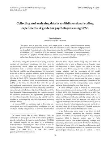
27Figure 1. Upper panel: data matrix containing intercity distances for 10 U.S. cities. Lower panel: optimal two‐dimensionalconfiguration computed by SPSS ALSCAL.Derived Stimulus ConfigurationEuclidean distance model1,0seattle,8new york,6chicago w ashingt,4,2denver,0sanfrancatlantaDimension 1,52,5Dimension 1hypotheses about these structures. Usually, MDS analysisstarts from data representing similarity scores betweenobjects, and tries to identify which dimensions could havebeen used for object comparison, for instance. MDS can alsobe used to test the validity of hypotheses about specificpsychological measures used in differentiating objects(Broderson, 1968, in Borg & Groenen, 1997), and identifysignificant object groupings.In the present paper, the basics of collecting andanalyzing similarity data are described. The first sectionfocuses on data collection methods and experimental designin general, while the second section concentrates onprogram use and output interpretation.Experimental designCollecting dataPractically any matrix of data, representing individualdegrees of relation between items, can be used in MDS,those of interest for cognitive psychologists being primarilysimilarities and dissimilarities (of course), rank‐orders, andconfusion data. The exact MDS model to be used isinfluenced by the goal of the analysis, but is mainlydetermined by the data set’s characteristics (which aredefined later in the text).Different psychological tasks can be used to collectsimilarity data. In the most common experimental task,namely pairwise comparison (as used in Shin & Nosofsky,1992), participants are asked to judge the resemblance or
28difference between two objects which are presentedsimultaneously or sequentially. They are often instructed torespond by moving a cursor to the desired position on acontinuous visual scale defining a similarity continuum.This is called the graphic rating method (Davison, 1983).Another way of collecting these judgments is to askparticipants to report the perceived similarity level using achoice of discrete numbers from a predefined scale. Forexample, in a pairwise comparison task, the number “1”could mean “highly similar”, while the number “9” wouldmean “highly dissimilar”, and all discrete numbers inbetween would represent various levels of similarity.Because the possible answers are limited in number anddiscrete, this is called the category rating method of collection(Davison, 1983).In magnitude estimation tasks (Stevens, 1971), a certainstimulus pair is chosen as a standard on each trial. Each ofthe remaining pairs of stimuli is to be judged against thestandard, in a relative way. For example, if the objects froma given pair look four times as dissimilar as the standard,the participant would give “4” as an answer, and if anotherpair looks half as dissimilar as the standard pair, theparticipant would give “1/2” as an answer. The estimateddissimilarity of a specific pair is equal to the geometric meanof all the judgments assigned to it by different participants.Therefore, only one matrix of dissimilarities is produced,whatever the number of participants.Another variant which uses a standard is the conditionalrank‐ordering task (see Schiffman et al., 1981; also called theanchor stimulus method, Borg & Groenen, 1997): for eachround of trials, all stimuli are presented simultaneously, anda single stimulus is chosen as a standard. The participant isasked to determine which other stimulus from the set ismost similar to the standard. This stimulus is given thehighest rank, and is removed from the set. In an iterativefashion, the participant must decide which remainingstimulus is now most similar to the standard, until allstimuli have been ranked. The standard, which is chosenrandomly, must be different for each round of trials, so thatat the end of the experiment, every stimulus has played thatrole. Ranking can also be constraint‐free. For that purpose,each object pair is typically presented on a card. Theparticipant is then asked to sort these cards so that the mostsimilar object is on top of the card stack and the mostdissimilar one at the bottom.In a free sorting task, a participant is presented with allstimuli simultaneously, and is asked to divide the set in anundefined number of subsets containing objects that appearsimilar in some sense. At the end of the task, two objectsfrom the same group are given a similarity of “1”, asopposed to stimuli from different groups, who are given ascore of zero. One has to be careful with this tasks, since thewell‐known fact that participants naturally tend to judgeinter‐object similarity using very few attributes could lead toa very low number of subsets (see Ahn & Medin, 1992;Regehr & Brooks, 1995).A related task is the category sorting task (Davison, 1983).Here, each possible pair of stimuli is printed on a separatecard. Participants must classify pairs in a specified numberof groups each representing a specific level of similarity.Once the task has been achieved, each pair is given a scoreaccording to its similarity category membership. Forexample, pairs from the “highly similar” category are giventhe lowest ranking score, “1”, while pairs from the “highlydissimilar” group are given a rank equal to the number ofpredefined categories. The experimenter can decide toconstrain the number of cards per group, and ask that all thegroups contain at least one card to avoid use of too fewsimilarity levels.Finally, when few stimuli are used, discrimination andidentification tasks can provide indirect similarity measures.The logic behind these two tasks is that as two items aremore and more similar, they should be more and moredifficult to discriminate. Hence, stimulus confusability canbe used as a measure. Stimulus‐stimulus confusions indiscrimination tasks occur when a participant is presentedwith a pair of different stimuli and asked if the two stimuliare the same or different. The number of “same” responsesto “different” pairs is the measure of confusability (andindirectly, of similarity) for a given pair of stimuli.Experimental design issuesSimilarity or dissimilarity?For technical reasons, most authors (such as Young &Harris, 2004) encourage the use of dissimilarities as input tothe MDS program, because their relationship to distances isdirect and positive (that is, the higher the dissimilarity, thelarger the perceived psychological distance). If similaritieshave been collected, Kruskal & Wish (1978) recommend thatthey be transformed by substracting the original data valuesfrom a constant which is higher than all collected scores.Trial orderingIn a MDS task, stimulus ordering is subject to twoparticular problems, namely position and timing effects.Position effects occur when an item is too often in the sameposition of presentation within a pair (for instance, if itemsare presented simultaneously, it appears too often on the leftpart of the screen). Timing effects for a given stimulus occurwhen the pairs in which that stimulus appears are notequally spaced throughout the trial list. To avoid these
29effects, the scientist may choose to use Ross ordering (Ross,1934), a technique used to balance position and time effectsby explicit planning when the number of items to becompared is low. If this is not the case, random orderingshould then be used: there is however no guarantee thatposition and timing effects are avoided, but they are kept toa minimum over replications.where D equals the maximal anticipated number ofdimensions, and I represents the number of items used inthe experiment (MacCallum, 1979).Reducing the number of necessary judgmentsData LevelsIn multidimensional scaling, the more judgments arecollected for each stimulus pairs, the more points can be fitin an n‐dimensional space. An analysis with more pointsprovides a more robust and precise stimulus space. That iswhy researchers usually prefer obtaining completejudgment matrices from many participants. However, withn items, a complete square similarity matrix is composed ofn(n‐1) possible cells or comparisons (when excludingidentical pairs), and this number grows rapidly whenadding more stimuli. Because the number of producedstimulus pairs in a design may be too high to be judged by asingle participant, there are a few ways to reduce thisnumber that have been proposed. First, if theoreticallysupported, one may assume that judgments are symmetric:this reduces by one half the number of required trials. Thisassumption is actually taken for granted in mostpsychological experiments, even if it was never proven(Schiffman et al., 1981). To avoid unknown asymmetryeffects and respect acceptable ordering characteristics, theexperimental program may be made to “flip the coin” beforeeach trial to randomly determine the position of eachstimulus in the presentation (left or right if the items arepresented simultaneously, first or second if they arepresented sequentially).Second, pairs may be randomly distributed overparticipants, with the set of pairs judged by differentparticipants being either completely independent oroverlapping (in both cases, no pair should be excluded).With a large number of participants, these subsets can becreated in a random fashion (Spence & Domoney, 1974).This produces a robust result when using Classical MDS(CMDS), mainly because judgments are generally averagedover participants, and this produces a complete matrix, butis not recommended when using models with replications orweights (RMDS and WMDS). Missing data also leads to thisrobustness difference, and should be avoided at all costswhen not using CMDS.In all cases, the number J of recommended judgmentsper pair of stimuli used in the MDS analysis should be equalto:40 DJ ( I 1)With MDS, data matrices can be defined by consideringmany of their characteristics, namely their measurementlevel, shape, and conditionality. According to Coombs’(1964) data theory, generally speaking, there are four levelsof data measurement, which are ordered from the weakestto the most stringent. The first one is the nominal (orcategorical) level, where objects are simply sorted into alimited number of groups. This level of data is notrecommended for use unless the number of categories isquite large. With the ordinal level, objects are arranged inorder of magnitude, but the only available information istheir comparative ranking. No numerical relationship holdsbetween objects. When using the interval or ratio levels,objects are placed on a scale such that the magnitude of thedifferences between objects is shown by the scale. Thedifference between these levels is that while the ratio levelcan lead to relative differences (as in “object x is twice orthree times as large or fast as object y”), in the interval level,there is no absolute zero, which prevents this kind ofconclusion. In both types of measurement levels, however, aprecise difference between values is always the same,wherever it is situated on the scale (e.g. the differencebetween 20 and 50 is the same as the difference between 70and 100).Analyzing dissimilarity dataData and measurement characteristicsData shapesData shapes are twofold. Square data occurs when thesame objects are represented by the rows and columns of thematrix. This generally happens when all objects arecompared to each other. Hence, the number of rows andcolumns are identical. When the order of presentationwithin a trial has no effect, that is if the similarity betweenobjects a and b is the same whichever object is presentedfirst, then the data is said square symmetric. In the oppositecase, if the order of presentation affects the value ofsimilarity, the data is square asymmetric. Rectangular datausually occurs when the objects represented by the rows aredifferent than the ones represented by the columns. Anexample would be if the rows represented differentindividuals, and the columns different psychological testscores1 . By definition, rectangular data is asymmetric. In thispaper, emphasis is put on square data.
30Figure 2. Two‐dimensional Euclidian space. The Euclidiandistance between points i and j is the hypothenuse of thehypothetical right triangle.calculation becomes:2dijk w ka ( xia x ja ) 2a2dijkwhereis the squared Euclidean distance between pointsi and j for participant k, x ia and x ja are the respectivecoordinates of points i and j on coordinate a, and wka (0 wka 1) represents the weight given to dimension a byparticipant k. A higher weight on a given dimension has theeffect of stretching the stimulus space on that particulardimension, while a lower weight has the opposite effect,namely shrinking.Dimension 2jx j2d ijxi 2iThe metric vs. nonmetric distinctionxi1x j1Dimension 1Measurement conditionalityThe result of data collection is that a certain number ofsquare or rectangular dissimilarity matrices equal to thenumber of participants are obtained. Depending on the roleplayed by individual differences and the shape of the data,different conditionality statuses define measurement.Data is said to be matrix conditional if there arehypothesized individual differences. This means that datafrom a specific data matrix can meaningfully be compared toeach other, but cannot be compared to data from othermatrices. Data from direct similarity rating usually falls inthis category. Unconditional data matrices can bemeaningfully compared to each other. For example, if onewere to measure response times from confusion errors, thisobjective measure could be compared across participants.The Euclidian modelMDS algorithms such as SPSS ALSCAL use the Euclidianmodel as a basis to compute optimal distances betweenobjects in an n‐dimensional stimulus space. The relateddistance function, Euclidian distance, corresponds to oureveryday experience with objects (Schiffman et al., 1981). Itis derived from the Pythagorean Theorem, and is defined asthe length of the hypotenuse linking two points in anhypothetical right triangle (Figure 2). The distance functionfor a Euclidian stimulus space is given by:dij2 ( xia x ja ) 2a2ijwhere d is the squared Euclidean distance between pointsi and j, and x ia and x ja are the respective coordinates ofpoints i and j on axis a.If perceptual/cognitive differences in the use ofpsychological dimensions are assumed, the distanceTo create an n‐dimensional map of distances, MDSalgorithms must use a function to scale the originaldissimilarities into “disparities”, which are directlycomparable to the obtained distances from the analysis. Forthis purpose, two types of function may be used (Figure 3).Torgerson (1952) proposed the use of a linear function tomap the original data onto “disparities”:δ ij f sij asij b( )where δ ij is the calculated disparity between objects i and j,s ij is the original dissimilarity score for this pair of objects,and a and b are the slope and intercept of the linear function( a 0 ). An analysis using this transformation function iscalled metric MDS.Shepard (1962a, 1962b) later discovered that metricinformation could be recovered even with weaker, non‐metric data. He found that with rank‐order data, the choiceof a linear function was too stringent, and proposed the useof any positive monotonic function (not necessarily a linearone) as sufficient to achieve the analysis. A positivemonotone function is defined as a transformation whichrespects the rank order of the data, or more precisely wherethe following relationship is respected:( sij ) ( sik ) f ( sij ) f ( sik )where s ij is the original dissimilarity measured betweenobjects i and j, s ik is the original dissimilarity measuredbetween objects i and k, f is a positive monotonic function,f(sij) is equal to δ ij , the disparity between objects i and j, andf(sik) is equal to δ ik , the disparity between objects i and k. Ananalysis using this type of function is called nonmetric MDS.When using nonmetric Classical MDS, a singletransformation is used, while with nonmetric ReplicatedMDS, a different function is used for each different datamatrix. All models discussed in this paper can be used withboth function types.
31Figure 3. Left panel: example of a positive linear function. Middle panel: example of a positive monotonic function whichis not linear, namely the exponential functions. Right panel: example of a non‐monotonic 46810x0.20.40.6Defining specific MDS models 2Classical MDS (CMDS) is a model which uses only onematrix of raw or averaged data, which is matrix‐conditional.When using this model, the algorithm produces ahypothetical Euclidian stimulus space which matches theoriginal data as much as possible. The first step is totransform the original dissimilarities into disparities using alinear (l(S) – for metric MDS) or monotonic (m(S) ‐ fornonmetric MDS) function.The model equation to be fit by ALSCAL is then:T (S) D 2 SSEwhere S is the original dissimilarities matrix, T(S) is adisparity matrix stemming from the transformation T, equalto l(S) or m(S) depending on whether the data areinterval/ratio (metric MDS) or ordinal (nonmetric MDS), D2represents the squared Euclidian distances fit by ALSCAL,and SSE is the sum of squared errors between the distancesand disparities. CMDS is the less robust analysis, becausethe algorithm only gets to fit a number of points equal to thenumber of stimulus pairs (or less if the matrix is symmetricor if an incomplete data scheme has been used).In Replicated MDS (RMDS), several matrices of data areused. These data are usually defined as matrix conditional.Once again, only one stimulus space is produced. Becausesystematic response bias differences between participantsare included in the analysis (reflecting the different waysthey use the response scale), the first step is to determineseveral transformation functions, one for each dissimilaritymatrix. Once again, these transformations can be either alllinear or all monotonic, but within these constraints, can allbe different. All matrices are judged to be linearly ormonotonically related, except for error. The model equationto be fit by ALSCAL is then:Tk (Sk ) D 2 SSEk0.81x0.511.522.53xwhere Sk is the original dissimilarities matrix for participantk, Tk(Sk) is an individual disparities matrix for participant kstemming from a unique transformation Tk, once again equalto lk(Sk) or mk(Sk) depending if the analysis is metric or nonmetric. D2 represents the squared Euclidian distances fit byALSCAL for the common stimulus space, and SSEk is thesum of squared errors between the distances and disparitiesfor participant k. RMDS is far more robust than CMDS,because the algorithm can use an increased number ofpoints, stemming from the fact that all data from all matricesare used in the analysis.The last type of MDS explored in this paper is WeightedMDS (WMDS – also known as Individual differences scalingor INDSCAL). In this type of analysis, SPSS ALSCALprovides the usual stimulus space, but also a participantspace which indicated the differential weighting given todimensions in the common stimulus space by eachparticipant, and the models fit to each participant’s data. Inthis model, several matrices of either matrix‐conditional orunconditional data are used. In WMDS, any twoparticipants’ personal distances need not be related by anylinear or monotonic function. The model equation to be fitby ALSCAL is then:Tk (Sk ) D k2 SSEkwhere S is the original dissimilarities matrix for participantk, Tk(Sk) is an individual disparities matrix for participant kstemming from a unique transformation Tk, once again equalto lk(Sk) or mk(Sk) depending if the analysis is metric or nonmetric. D k2 represents the squared Euclidian distances fit byALSCAL for participant k, and SSEk is the sum of squarederrors between the distances and disparities for participantk. The distances are found in participant k’s personalstimulus space, which can be recovered by applying thepersonal weights to the common distance space, as in:X k XWk1 / 2
32Table 1. Decision table relating data characteristics to their appropriate MDS modelShape of data?SquareNumber of matrices?Perceptual/cognitivedifferences assumed?MeasurementConditionality?Data level?MDS ModelOneSeveralN/ANoUnconditionalIntervalor RatioMetricCMDSOrdinalor alor Ratioor IntervalOrdinalor Ratioor NominalMetricNonmetricWMDSWMDSNote. To find the appropriate model, one must answer all questions sequentially, from top to bottom. For example, ifworking with several square matrices of interval data, where no perceptual/cognitive differences are assumed, the user’spath would be “SquareöSeveralöNoöMatrix conditionalöInterval or Ratio, and the reader should conclude that theuse of metric RMDS is appropriate.where Xk is the coordinate matrix representing participantk’s stimulus space, X is the coordinate matrix from thecommon stimulus space, and Wk is the weight matrix forparticipant k. WMDS possesses the robustness of RMDS, butalso provides some flexibility, because the stimulus spacedoes not have to “directly” fit every matrix of data.The reader is encouraged to use Table 1 to determine theexact MDS model needed for the analysis, depending on theshape and level of the data, the number of similaritymatrices used in the analysis, the measurementconditionality, as well as the decision to take into accountpsychological differences between participants.Syntax useTo achieve an MDS analysis, the data must firstbe entered in matrix fashion in an SPSS data file.Figure 4 shows an example file with threehypothetical data matrices. Each matrix representsthe similarity judgments collected for one participant(subject). For identification purposes, the subjectnumber is put in the first column, along each line ofthis participant’s data matrix. However, whenentering many square matrices, no identifier has tobe provided for each matrix; ALSCAL achieves thefile separation by itself. Each column’s variablename (object1, object2, object3, object4) is attributed tothe compared object’s identity. These variable nameswill be used as identifiers in the output and graphs.As can be seen, when considering that the data aresymmetric (as is the case here), one does not need toenter data above the matrix diagonal (nor on thediagonal for that matter, because any object isalways minimally dissimilar to itself). Whenentering many matrices, no identifier has to be provided foreach matrix; ALSCAL achieves the file separation by itself.Using this file, the user can produce different RMDS orWMDS, assuming that the data are eitherTo use the ALSCAL procedure in SPSS syntax, the usermust enter the ALSCAL command, followed by the list ofvariables (names of the data columns), in the followingfashion:ALSCAL VARIABLES v1 to vnwhere v1 represents the first column of data, and vnrepresents the last one. Following this command, manyFigure 4. SPSS file representing three data matrices. Each matrix contains inter‐object dissimilarity judgments. The reader is encouraged to analyze theexample data using the corresponding file found on the journal’s website(www.tqmp.org), and the code examples from Table 2.
33Table 2. Default values and typical examples of syntax fordifferent MDS modelsDefault values/SHAPE SYMMETRIC/LEVEL ORDINAL/CONDITION MATRIX/MODEL EUCLID/CRITERIA CUTOFF(0) CONVERGE(.001)ITER(30) STRESSMIN(.005)DIMENS(2)/PRINT DATA/PLOT DEFAULTMetric CMDS or RMDSALSCAL VARIABLES v1 to vn/LEVEL INTERVAL or RATIO/CRITERIA DIMENS(1,6)/PRINT DATA HEADER/PLOT DEFAULT ALL.Metric WMDSALSCAL VARIABLES v1 to vn/LEVEL INTERVAL or RATIO/MODEL INDSCAL/CRITERIA DIMENS(2,6)/PRINT DATA HEADER/PLOT DEFAULT ALL.Note. When achieving a nonmetric analysis, the LEVELsubcommand values are ORDINAL or NOMINAL. InWMDS, note that the minimal dimensionality is always 2.Any block of syntax in SPSS must end with a period; else theprogram is not executed.subcommands can be entered to specify the type of analysisneeded, and other necessary criteria. Each subcommandmust be preceded by a backslash. Examples of typical syntaxblocks for different MDS types are detailed in Table 2.The first subcommand is SHAPE, which describes theshape of the data. The eligible values are SYMMETRIC (forsquare symmetric data), ASYMMETRIC (for squareasymmetric data), and RECTANGULAR. The followingsubcommand concerns the LEVEL of the data. It determinesif the algorithm should use a metric or nonmetrictransformation function. The values which can be enteredare ORDINAL, INTERVAL, RATIO and NOMINAL.Measurement conditionality is defined by the CONDITIONsubcommand, which takes the values MATRIX (for matrix‐conditional data), ROW (for row‐conditional data), orUNCONDITIONAL. Next is the MODEL subcommand. Fiveoptions are available, but the user usually limits himself tothe basic Euclidian model (represented by the valueEUCLID) or the Individual differences scaling model (forwhich the appropriate value is INDSCAL). 3The CRITERIA subcommand is special, because it iscomposed of many parameters, for which different valuesmust be provided. For each parameter, the wanted valuesmust be inserted between parentheses. The first parameter isthe CUTOFF, which specifies the lower bound for the scoresfound in the data matrices. By default, this is left at zero(“0”), so that only negative scores are eliminated. The threenext parameters provide a disjunctive stopping rule for thealgorithm (i.e. as soon as the algorithm reaches a criticalvalue for one of the parameters, the fitting procedure ends).CONVERGE represents the minimal S‐STRESS (a measuredefined in the next section) improvement needed for asupplemental iteration. ITER defines the maximal number ofiterations for the analysis. Finally, STRESSMIN defines aminimal cutoff for the S‐STRESS value. For a given iteration,if the value is equal to or lower than the cutoff, the program
Collecting and analyzing data in multidimensional scaling experiments: A guide for psychologists using SPSS Gyslain Giguère Université du Québec à Montréal This paper aims at providing a quick and simple guide to using a multidimensional scaling procedure to analyze experimental data. First, the operations of data collection and preparation