WIXLIB

By contrast, efforts to understand graduate and professional school affordability have lagged greatly. The mostdeveloped of these approaches tends to be for law school. The Access Group, in its 2015 report A Framework forThinking About Law School Affordability vii, explicitly considered law school differences, geographic andemployment differences, and individual differences to conclude that in many cases, the earnings premium doesnot justify the investment. However, others are more optimistic about the environment for law students, such asSimkovic and McIntyre (2014)viii, who estimate a lifetime earnings premium for a law degree at 1 million or more.Analyses for other first-professional degrees appear to be inadequate.To date, this benchmark has not been formally operationalized, even though a recent study by the Institute forHigher Education Policy did use the Rule of 10 to compare affordability for various “typical” student against(typical, aggregated) net prices for institutional sectors. This simulation suggested that for all but the highestincome families, most colleges are unaffordable based on the Rule of 10.ix Importantly, IHEP recognized thataffordability is not a binary metric, but should be contextualized to estimate individual goals and circumstances,including geography and personal lifestyle. This crucial perspective is also reflected in our study.We aim to understand the socioeconomic and demographic characteristics of debt accrual and how debt incurredduring professional education affects a proposed definition of affordability. HelioCampus’ approach to datamodeling and analysis allows us to incorporate two novel features into this study. First, using unit record level filesallows us to model affordability in a retrospective fashion for individual students, rather than hypothetical or“average” students. Second, we apply this model to professional degree programs, in which students typically andwillingly incur very high levels of debt with the expectation that this debt will be dischargeable within a reasonabletime based on the high earnings associated with these degrees.DeliverablesTo provide a robust picture of affordability for UMB and its constituent schools, HelioCampus leveraged itsexpertise in data modeling, analysis, and visualization to provide the following products. The focal programs in allof these products included Nursing (Bachelor’s and Master’s); Social Work (Master’s); Medical, Pharmacy, Law,Dental.1) Affordability Data ModelIn collaboration with subject matter experts at UMB, HelioCampus identified the appropriate data sources andelements therein to support an analysis of debt and affordability. These sources included historical census files(enrollment, degree, and financial aid) and debt at graduation across programs spanning a 10-year time frame.Our data engineers combined these files into a single Graduate Extract that was used to analyze debtcharacteristics.We then developed a Wage Extract using Occupational Employment Statistics data from the U.S. Bureau ofLabor Statistics (resolved to the state level) and Maryland Department of Labor, Licensing and RegulationQuarterly Census of Employment and Wages, resolved at the county and Workforce Investment Area level, whichcomprises economically similar counties.These two data sets were then combined to generate an Affordability Extract (Fig. 1). The critical linking functionused to join these two sources was the Classification of Instructional Programs (CIP) code, which links to bothinstructional programs in the former extract and occupational codes in the latter.Contains confidential and proprietary information of HelioCampus. Use of these materials is limited to HelioCampus licensees,and is subject to the terms and conditions of one or more written license agreements between HelioCampus and the licenseein question.4

Figure 1. Structure of the Affordability Extract.2) DashboardsFollowing data analysis, HelioCampus developed a series of dashboards that provided an overview of patternsand trends in enrollment, degree recipients, and debt and repayment rates. Details of repayment rate calculationsare included in the technical appendix. Understanding student debt and repayment is the foundation on which theAffordability Estimator dashboard is based.a. Historical Trends of Cost of Attendance, Financial Aid Awards, Student Debt and other UMB keymetrics.b. Benchmarking Metrics for UMB against a selected peer group for Tuition and fees, Financial Aid,Student Debt, Diversity, and other key metrics.c. Affordability Trends broken out by school, program and student attributes.3) Project summary & roadmap for future workAt the outset, it was clear that significant roadblocks would be present in the form of sparse or unobtainable data.Defining and articulating these data deficiencies, and suggesting approaches to work around these deficiencies,is a key goal of this work.The HelioCampus Analytic StrategyWhile the Lumina Foundation correctly note that unmet need and Expected Family Contribution are limited in theirutility to estimate or parameterize affordability, their work is focused in scope to the cost of education. As theirwork implicitly recognizes, however, the fundamental driver of affordability is student debt.We can decompose affordability into two basic equations.The affordability condition exists where1)Cost of Education ([10% of discretionary income] [10 years]) [10 hours/week in-school employment]Contains confidential and proprietary information of HelioCampus. Use of these materials is limited to HelioCampus licensees,and is subject to the terms and conditions of one or more written license agreements between HelioCampus and the licenseein question.5

As shown in the IHEP study, this condition does not hold for the vast majority of college attendees. Thedifference, then, is accounted for by loans, which means that students graduate with debt. This debt can bedefined as2) Student Debt [Cost of education] ‒ [financial aid] ‒ [Monetary contributions from work/family].Knowing accurately at the student level how much debt a graduate has when they begin their career allows us toestimate how they might repay their debt. But we also need to understand how the debt is repaid, and whatcorrelates exist with debt accrual and repayment. Therefore, we use in a three-pronged approach. First, wevisually and statistically analyze actual total debt at graduation to understand-What are debt levels at graduation across programs?-What student characteristics correspond to debt level?-How many students graduate without debt, and what features do these graduates exhibit?Second, we leverage the National Student Loan Data System to capture current debt among a representativesubsample of graduates. This provided a cross section of graduates from across programs over a range of timesince graduation. We used these data to ask-What is the typical time to repayment, and how does it vary?-What is the typical rate of repayment, and does this vary across programs and over time?-Are rates of repayment constant in terms of amount repaid and proportion of debt repaid?Third, we used the insights gained from these exercises to develop an Affordability Estimator, incorporatingstudent debt and demographic characteristics with official state and federal wage data to understand under whatconditions a degree would be considered affordable. The tool is a robust and flexible, and helps to answer forwhom and where a degree is affordable.The Foundation of Affordability: Student DebtCollege affordability has become a prominent issue because of the rapid increase in the cost of attendance. It hasbeen amply documented that the increase in college tuition has far outpaced wages and inflation over the pastfew decades. For public four-year institutions, the inflation-adjusted total cost of attendance increased more thanhalf between 2006 and 2016x. Even in the state of Maryland, which has historically consistently supported highereducation, tuition and fees have increased roughly 3% per year in recent years xi, compared with medianhousehold income that has been consistently lower.The unique structure of UMB, where individual professional schools have greater autonomy and latitude in coststructure (within the constraints set by USM), results in greater variability in cost structure and potentially greaterincreases in some Schools than others.As shown in Fig. 2, the cost of attendance for professional school students has increased at a fairly consistentrate, with the School of Dentistry increasing the most from 2011-2016.Contains confidential and proprietary information of HelioCampus. Use of these materials is limited to HelioCampus licensees,and is subject to the terms and conditions of one or more written license agreements between HelioCampus and the licenseein question.6

Figure 2. Trends in educational expenses among professional schools.However, even though the cost of attendance has escalated, average levels of student debt at graduation haveincreased at a much lower rate, and in a few cases, have actually declined over the same time period (Fig. 3).Contains confidential and proprietary information of HelioCampus. Use of these materials is limited to HelioCampus licensees,and is subject to the terms and conditions of one or more written license agreements between HelioCampus and the licenseein question.7

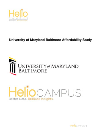
Figure 3. Trends in student debt at graduation.Still, there is a high level of disparity in which students accrue the most debt. Graduates of the School ofDentristry accumulate significantly more debt than students from any other school. There is little evidence forsystematic gender-based difference in debt load.Conversely, there is a tremendous racial disparity in debt at graduation. Underrepresented minorities, andespecially African American graduates have consistently far greater debt level than their fellow graduates. Fig. 4shows these debt levels by color, with relative number of graduates indicated by the size of each square. Themost dramatic disparity occurs for Law School graduates, where African Americans on average can expect tograduate with 55% greater debt than their white counterparts. African American School of Dentristry graduateshave the dubious distinction of graduating with the greatest amount of debt, averaging 218,000.Contains confidential and proprietary information of HelioCampus. Use of these materials is limited to HelioCampus licensees,and is subject to the terms and conditions of one or more written license agreements between HelioCampus and the licenseein question.8

Figure 4. Debt levels at graduation by professional school and ethnicity. Color indicate amount of debt, and symbols sizecorresponds to the number of graduates in that category.The other major component of debt levels at graduation is the level of education of the parents. While this effect issmall across all schools, it is particularly keen for School of Dentistry students, where graduates whose parentsattended college incurred 31,000 less debt on average than their counterparts whose parents did not attendcollege.This pattern persisted for those students graduating with no debt: 8% of students whose parents did not attendcollege graduated with no debt, vs. 13% of students whose parents attended college. Within-program disparitieswere not notable.In general, based on raw debt accumulated, Dental School and minority graduates are at the forefront of facingthe issue of high debt. Conversely, Pharmacy and Physical Therapy students tend to face much lower debtobstacles upon entering their professional careers.Operationalizing Affordability: Debt RepaymentRegardless of the total amount of debt a student graduates with, that debt must still be paid down eventually. Howa graduate pays down this debt will certainly reflect numerous choices a graduate makes, including geographic,family, and professional considerations. The range of possibilities is vast; before delving into these lifestylefactors, though, it is useful to understand broad patterns of repayment rates, both absolute and relative to totaldebt.We submitted 450 names to NSLDS of graduates with debt from the programs of interest to identify the amountthe currently still owe. These 450 graduates were distributed proportionally across the graduating classes of 2011through 2015 and across the programs of interest. Using these values, we estimated absolute per year repaymentContains confidential and proprietary information of HelioCampus. Use of these materials is limited to HelioCampus licensees,and is subject to the terms and conditions of one or more written license agreements between HelioCampus and the licenseein question.9

rate as [initial debt - remaining debt]/years since graduation, and proportional repayment rate (repayment ratio) as([initial debt – remaining debt] /initial debt)/years since graduation.Within each program, rates of change of repayment rate and repayment ratios were shallow, allowing us tocompare these consistent repayment metrics across programs and demographic features. Similar to debtaccrued, repayment rate was significantly greater for Dental School graduates; Pharmacy School graduates alsorepaid debt at higher levels per year than other programs. Notably, the former also had the highest total debt,whereas the latter was similar to other programs.These disparities in debt and repayment, however, do not extend to repayment behavior; graduates on averagerepaid their debt at an average of 8-13% per year. Even for those programs where repayment may be delayeddue to the professional pathway (e.g. MD graduates progress through residencies and internships) or careerchoices (many JD graduates obtain employment in the public sector or take on clerkships), there are relatively lowamounts of variation. The result of this is that debt clearance among UMB graduates sits at 30% after 7 years,the longest time period available for this data set. Pharmacy School graduates had a 38% payoff rate at 7 years,highest among all programs.Finally, we modeled debt “survival” to estimate the predicted interval-specific likelihood of debt fulfillment.Although the number of data points available for residual debt was generally too low for sufficient statistical powerto see an effect, patterns were similar to those seen across other analyses. Pharmacy graduates had a 52%predicted expectation of retiring debt at 7 years, and graduates of the dental program had just a 36% likelihood.Other programs hovered 40%.Along with total debt and other features, minorities showed a striking (and significant) gap in likelihood to repay.Underrepresented minorities had a predicted likelihood of repayment of just 17%, compared to 47% for nonminorities.Affordability in Real Life: The Affordability EstimatorRetrospectively, there are consistent and clear patterns in debt accumulation and repayment. For various otherstakeholders, a retrospective point of view may not be sufficient. Campus and program leaders are keenlyinterested in where their students are coming from, and where they go after graduation. Policy makers need toensure that the critical functions provided by graduates can be filled without regard to geographic constraints. Andthe most important constituents, students (and prospective students) need to know the extent to whicheducational debt may constrain them in geographic, professional, and lifestyle choices.Repayment of debt is based on the amount of discretionary income available to an individual. Estimatingrepayments prospectively, even using historical data, is difficult because of the uncertainty in definingdiscretionary income. In the Lumina Foundation model, discretionary income was defined as anything over 200%of poverty level. Certainly, this constraint is unnecessarily narrow for almost all graduated of UMB professionalschools. Furthermore, we recognize that, while fairly consistent, there are numerous examples of (non-statistical)outliers for both debt and repayment. It is critical to account for this variation.We therefore developed a tool that allows for maximum flexibility. The user is able to choose wage, salary, anddiscretionary-income levels based on what most accurately reflects their educational plans and professionalgoals, in addition to using “typical” or custom debt levels. Wage Benchmark: Using data from BLS and MD DLLR, the user can choose from a range of wagequantiles (specific for the occupational category of interest) corresponding to national or state-levelwages.Salary Benchmark: Entry-position benchmark salaries can be selected from quantiles specific toWorkforce Investment Area (MD multi-county areas) wages.Contains confidential and proprietary information of HelioCampus. Use of these materials is limited to HelioCampus licensees,and is subject to the terms and conditions of one or more written license agreements between HelioCampus and the licenseein question.10

Discretionary Income: We define discretionary income as the difference between the Salary Benchmarkand the Wage Benchmark. Selecting low values for the Wage Benchmark and high values for SalaryBenchmark results in higher discretionary income, all else being equal. The user selects the proportion ofdiscretionary income to dedicate to debt repayment.Debt: The user can select a default debt level reflecting the median debt of the most recent graduatingclass (for the program in question), or custom debt levels.Occupation: The professional degrees offered by UMB typically correspond to multiple federaloccupational codes. The Affordability Estimator allows the user to select a single occupation or compareacross multiple occupations.The output (Fig. 5) shows debt paid (yearly and cumulatively) on a biennial basis over 20 years, along with totalremaining debt. For scenarios in which remaining debt reaches zero, that set of conditions is classified as“Affordable.” The relative affordability of Maryland counties and Workforce Investment Areas is visualized to assistin understanding potential geographic constraints and disparities.Figure 5. Representative sample output of the Affordability Estimator.Contains confidential and proprietary information of HelioCampus. Use of these materials is limited to HelioCampus licensees,and is subject to the terms and conditions of one or more written license agreements between HelioCampus and the licenseein question.11

Affordability Case StudiesBecause of the numerous possible permutations of inputs, we provide examples of how the Affordability Estimatormight be used in practice.Example 1. Physical TherapyFor a hypothetical graduate with a “typical” debt set at the default amount of 115, 755. As a starting point, we setthe Reference Salary to the state median for the occupation. (There are two shown in Fig. x, of five available thatalign with this degree.) Assuming a somewhat high demand for Occupational and Physical Therapists, the startingsalary is set at the 75th percentile. A reasonable first pass for a typical graduate is 30% of discretionary income(depending on the county, this is generally 5,000 per year or less.)This analysis (Fig. 6) shows that, under these conditions: a high degree of geographic variation existsoccupational therapy is relatively more affordable across a wider geographic rangethe lower Eastern Shore is not particularly affordable, particularly as a Physical Therapistthe upper Eastern Shore and northern MD are (perhaps surprisingly) affordablea large swath of central MD exhibits low affordabilityWhile not shown, increasing the proportion of discretionary income dedicated to debt repayment to 50% revealsthat essentially all of MD is now affordable for Occupational Therapists, and most of MD is now affordable forPhysical Therapists (with the notable exception of the lower Eastern Shore). The nature of interplay betweenmultiple variables allows us to see nonintuitive patterns that would otherwise be inscrutable without the visualapproach used in the Affordability Estimator.Figure 6. Affordability map for DPT graduates, showing Physical Therapist and Occupational Therapist.Contains confidential and proprietary information of HelioCampus. Use of these materials is limited to HelioCampus licensees,and is subject to the terms and conditions of one or more written license agreements between HelioCampus and the licenseein question.12

Example 2. PharmacyThere is a striking disparity between affordability seen for the DPT and for Pharmacy graduates. Under identicalconditions of debt levels and repayment rates, most of the state falls into the “affordable” classification (Fig. 7).Both western Maryland and the lower Eastern Shore are now affordable, whereas the upper Eastern Shore ismuch less so. There are several implications to these patterns: Currently affordable areas may experience a glut of graduates seeking to capitalize on this geographicdifference in affordability.Those areas that are less affordable may conversely see a dearth of pharmacists, resulting in greaterdemand, higher wages, and eventually greater affordability.From an institutional perspective, it may be reasonable to review tuition and fees for this program tonormalize a program that appears very affordable, or alternatively highlight program afford

Dental. 1) Affordability Data Model In collaboration with subject matter experts at UMB, HelioCampus identified the appropriate data sources and elements therein to support an analysis of debt and affordability. These sources included historical census files