WIXLIB

IEEE TRANSACTIONS ON PATTERN ANALYSIS AND MACHINE INTELLIGENCE, VOL. XX, NO. XX, JUNE 2011kernelHellinger’sχ2k(x, y) xyxy2 x ysignature min{x, y}e λ /221π 1 4ω 23λx2JSlog2 x yx y2k(x, 0.25)1K(λ)00.6χ2inters.JS100.4 31010χ2intersectionJS0.210.2 2 20.5x0.80 110100Ψω(x)κ(ω)20.60.402 sech(πω)log 4 1 4ω 21010Hellinger’sχ2intersectionJS0.8 log2 1 e λ λ e 2log2 1 eλ2e22log2 x yyfeature Ψω (x) xpeiω log x x sech(πω)q1eiω log x 2xπ 1 4ω 2q2x sech(πω)eiω log x log4 1 4ω 205λχ2intersectionJS 4101000.51ω1.502 0.201ω23Fig. 1. Common kernels, their signatures, and their closed-form feature maps. Top: closed form expressions forthe χ2 , intersection, Hellinger’s (Battacharyya’s), and Jensen-Shannon’s (JS) homogeneous kernels, their signaturesK(λ) (Sect. 2), the spectra κ(ω), and the feature maps Ψω (x) (Sect. 3). Bottom: Plots of the various functions for thehomogeneous kernels. The χ2 and JS kernels are smoother than the intersection kernel (left panel). The smoothnesscorresponds to a faster fall-off of the the spectrum κ(ω), and ultimately to a better approximation by the homogeneouskernel map (Fig. 5 and Sect. 4.2).the kernel signature.Stationary kernels. A kernel ks : R R R is calledstationary (or translation invariant, shift invariant) if c R :ks (c x, c y) ks (x, y).(4)By choosing c (x y)/2 a stationary kernel can berewritten as y x x y,ks (x, y) ks (c x, c y) ks22(5) K(y x),where we also call the scalar function λ λ, λ R.K(λ) ks22(6)the kernel signature.Any scalar function that is PD is the signature of akernel, and vice versa. This is captured by the followingLemma, proved in Sect. 10.2.Lemma 1. A γ-homogeneous kernel is PD if, and only if,its signature K(λ) is a PD function. The same is true forstationary a stationary kernel.So far homogeneous and stationary kernels k(x, y)have been introduced for the scalar (D 1) case. Suchkernels can be extended to the multi-dimensional caseby either additive or multiplicative combination, which aregiven respectively by:K(x, y) DXl 1k(xl , yl ), or K(x, y) DYk(xl , yl ). (7)l 1Homogeneous kernels with negative components. Homogeneous kernels, which have been defined on thenon-negative semiaxis R 0 , can be extended to the wholereal line R by the following lemma:Lemma 2. Let k(x, y) be a PD kernel on R 0 . Then theextensions sign(xy)k( x , y ) and 21 (sign(xy) 1)k( x , y )are both PD kernels on R.Metrics. It is often useful to consider the metric D(x, y)that corresponds to a certain PD kernel K(x, y). This isgiven by [32]D2 (x, y) K(x, x) K(y, y) 2K(x, y).(8)2Additive and multiplicative combinations. In applications one is interested in defining kernels K(x, y) formulti-dimensional data x, y X D . In this paper Xmay denote either the real line R, for which X D isthe set of all D-dimensional real vectors, or the nonDnegative semiaxis R is the set of all0 , for which XD-dimensional histograms.Similarly d (x, y) will denote the squared metric obtained from a scalar kernel k(x, y).2.1Examples2.1.1 Homogeneous kernelsAll common additive kernels used in computer vision,such as the intersection, χ2 , Hellinger’s, and Jensen-

IEEE TRANSACTIONS ON PATTERN ANALYSIS AND MACHINE INTELLIGENCE, VOL. XX, NO. XX, JUNE 2011Shannon kernels, are additive combinations of homogeneous kernels. These kernels are reviewed next andsummarized in Fig. 1. A wide family of homogeneouskernel is given in [29].Hellinger’s kernel. The Hellinger’s kernel is given by k(x, y) xy and is named after the corresponding additive squared metric D2 (x, y) k x yk22 which isthe squared Hellinger’s distance between histograms xand y. This kernel is also known as Bhattacharyya’s coefficient. Its signature is the constant function K(λ) 1.Intersection kernel. The intersection kernel is given byk(x, y) min{x, y} [33]. The corresponding additivesquared metric D2 (x, y) kx yk1 is the l1 distancebetween the histograms x and y. Note also that, byextending the intersection kernel to the negative realsby the second extension in Lemma 2, the correspondingsquared metric D2 (x, y) becomes the l1 distance betweenvectors x and y.χ2 kernel. The χ2 kernel [34], [35] is given by k(x, y) 2(xy)/(x y) and is named after the correspondingadditive squared metric D2 (x, y) χ2 (x, y) which isthe χ2 distance. Notice that some authors define the χ2kernel as the negative of the χ2 distance, i.e. K(x, y) χ2 (x, y). Such a kernel is only conditionally PD [18],while the definition used here makes it PD. If the histograms x, y are l1 normalised, the two definitions differby a constant offset.Jensen-Shannon (JS) kernel. The JS kernel is givenby k(x, y) (x/2) log2 (x y)/x (y/2) log2 (x y)/y.It is named after the corresponding squared metricD2 (x, y) which is the Jensen-Shannon divergence (orsymmetrized Kullback-Leibler divergence) between thehistograms x and y. Recall that, if x, y are finiteprobability distributions (l1 -normalized histograms), theKullback-Leibler divergence is given by KL(x y) Pdl 1 xl log2 (xl /yl ) and the Jensen-Shannon divergenceis given by D2 (x, y) KL(x (x y)/2)) KL(y (x y)/2)). The use of the base two logarithm in the definition normalizes the kernel: If kxk1 1, then K(x, x) 1.γ-homogeneous variants. The kernels introduced sofar are 1-homogeneous. An important example of 2homogeneous kernel is the linear kernel k(x, y) xy.It is possible to obtain a γ-homogeneous variant of any1-homogeneous kernel simply by plugging the corresponding signature into (2). Some practical advantagesof using γ 6 1, 2 are discussed in Sect. 8.2.1.2 Stationary kernelsA well known example of stationary kernel is the Gaussian kernel ks (x, y) exp( (y x)2 /(2σ 2 )). In lightof Lemma 1, one can compute the signature of theGaussian kernel from (6) and substitute it into (3) toget a corresponding homogeneous kernel kh (x, y) 2xy exp( (log y/x) /(2σ 2 )). Similarly, transforming the2homogeneous χ kernel into a stationary kernel yieldsks (x, y) sech((y x)/2).2.24NormalizationEmpirically, it has been observed that properly normalising a kernel K(x, y) may boost the recognitionperformance (e.g. [36], additional empirical evidence isreported in Sect. 8). A way to do so is to scale thedata x X D so that K(x, x) const. for all x. Inthis case one can show that, due to positive definiteness,K(x, x) K(x, y) . This encodes a simple consistencycriterion: by interpreting K(x, y) as a similarity score, xshould be the point most similar to itself [36].For stationary kernels, ks (x, x) K(x x) K(0) shows that they are automatically normalized.For γ-homogeneous kernels, (2) yields kh (x, x) γ(xx) 2 K (log(x/x)) xγ K(0), so that for the corresponding additive kernel (7) one has K(x, x) PDγl 1 kh (xl , xl ) kxkγ K(0) where kxkγ denotes thelγ norm of the histogram x. Hence the normalisationcondition K(x, x) const. can be enforced by scalingthe histograms x to be lγ normalised. For instance, forthe χ2 and intersection kernels, which are homogeneous,the histograms should be l1 normalised, whereas for thelinear kernel, which is 2-homogeneous, the histogramsshould be l2 normalised.3A NALYTICFORMS FOR FEATURE MAPSA feature map Ψ(x) for a kernel K(x, y) is a functionmapping x into a Hilbert space with inner product h·, ·isuch that x, y X D : K(x, y) hΨ(x), Ψ(y)i.It is well known that Bochner’s theorem [7] can beused to compute feature maps for stationary kernels.We use Lemma 1 to extend this construction to the γhomogeneous case and obtain closed form feature mapsfor all commonly used homogeneous kernels.Bochner’s theorem. For any PD function K(λ), λ RDthere exists a non-negative symmetric measure dµ(ω)such that K is its Fourier transform, i.e.:ZK(λ) e ihω,λi dµ(ω).(9)RDFor simplicity it will be assumed that the measure dµ(x)can be represented by a density κ(ω) dω dµ(ω) (thiscovers most cases of interest here). The function κ(ω) iscalled the spectrum and can be computed as the inverseFourier transform of the signature K(λ):Z1eihω,λi K(λ) dλ.(10)κ(ω) (2π)D RDStationary kernels. For a stationary kernel ks (x, y) defined on R, starting from (5) and by using Bochner’stheorem (9), one obtains:Z ks (x, y) e iωλ κ(ω) dω, λ y x, Z pp e iωx κ(ω)e iωy κ(ω) dω.

IEEE TRANSACTIONS ON PATTERN ANALYSIS AND MACHINE INTELLIGENCE, VOL. XX, NO. XX, JUNE 2011Define the function of the scalar variable ω RpΨω (x) e iωx κ(ω) .(11)Here ω can be thought as of the index of an infinitedimensional vector (in Sect. 4 it will be discretized toobtain a finite dimensional representation). The functionΨ(x) is a feature map becauseZ Ψω (x) Ψω (y) dω hΨ(x), Ψ(y)i.ks (x, y) γ-homogeneous kernels. For a γ-homogenoeus kernelk(x, y) the derivation is similar. Starting from (2) and byusing Lemma 1 and Bochner’s theorem (9):Z γye iωλ κ(ω) dω, λ log ,k(x, y) (xy) 2x Z ppe iω log y y γ κ(ω) dω. e iω log x xγ κ(ω) The same result can be obtained as a special case ofCorollary 3.1 of [29]. This yields the feature mappΨω (x) e iω log x xγ κ(ω) .(12)Closed form feature maps. For the common computervision kernels, the density κ(ω), and hence the featuremap Ψω (x), can be computed in closed form. Fig. 1 liststhe expressions.Multi-dimensional case. Given a multi-dimensional kernel K(x, y) hΨ(x), Ψ(y)i, x X D which is aadditive/multiplicative combination of scalar kernelsk(x, y) hΨ(x), Ψ(y)i, the multi-dimensional featuremap Ψ(x) can be obtained from the scalar ones asΨ(x) DMΨ(xl ),l 1Ψ(x) DOΨ(xl )(13)l 1respectively for additive and multiplicative cases. Here is the direct sum (stacking) of the vectors Ψ(xl ) and their Kronecker product. If the dimensionality of Ψ(x) isn, then the additive feature map has dimensionality nDand the multiplicative one nD .4A PPROXIMATEDFEATURE MAPSThe features introduced in Sect. 3 cannot be used directlyfor computations as they are continuous functions; inapplications low dimensional or sparse approximationsare needed. Sect. 4.1 reviews Nyström’s approximation,the most popular way of deriving low dimensionalfeature maps.The main disadvantages of Nyström’s approximation is that it is data-dependent and requires training.Sect. 4.2 illustrates an alternative construction based onthe exact feature maps of Sect. 3. This results in dataindependent approximations, that are therefore calleduniversal. These are simple to compute, very compact,and usually available in closed form. These feature mapsare also shown to be optimal in Nyström’s sense.54.1 Nyström’s approximationGivan a PD kernel K(x, y) and a data density p(x), theNyström approximation of order n is the feature mapΨ̄ : X D Rn that best approximates the kernel at pointsx and y sampled from p(x) [19]. Specifically, Ψ̄ is theminimizer of the functionalZ 2E(Ψ̄) K(x, y) hΨ̄(x), Ψ̄(y)i p(x) p(y) dx dy.X D X D(14)For all approximation orders n the components Ψ̄i (x),i 0, 1, . . . are eigenfunctions of the kernel. SpecificallyΨ̄i (x) κ̄i Φ̄i (x) whereZK(x, y)Φ̄i (y) p(y) dy κ̄2i Φ̄i (x),(15)XDκ̄20 κ̄21 . . . are the (real and non-negative) eigenvalues in decreasing order,and the eigenfunctions Φ̄i (x)Rhave unitary norm Φ̄i (x)2 p(x)dx 1. Usually thedata density p(x) is approximated by a finite sample setx1 , . . . , xN p(x) and one recovers from (15) the kernelPCA problem [18], [19]:N1 XK(x, xj )Φ̄i (xj ) κ̄2i Φ̄i (x).N j 1(16)Operationally, (16) is sampled at points x x1 , . . . , xNforming a N N eigensystem. The solution yields Nunitary1 eigenvectors [Φ̄i (xj )]j 1,.,N and correspondingeigenvalues κ̄i . Given these, (16) can be used to computeΨ̄i (x) for any x.4.2 Homogeneous kernel mapThis section derives the homogeneous kernel map, auniversal (data-independent) approximated feature map.The next Sect. 5 derives uniform bounds for the approximation error and shows that the homogeneous kernelmap converges exponentially fast to smooth kernels suchas χ2 and JS. Finally, Sect. 5.1 shows how to selectautomatically the parameters of the approximation forany approximation order.Most finite dimensional approximations of a kernelstart by limiting the span of the data. For instance,Mercer’s theorem [37] assumes that the data spans acompact domain, while Nyström’s approximation (15)assumes that the data is distributed according to adensity p(x). When the kernel domain is thus restricted,its spectrum becomes discrete and can be used to derivea finite approximation.The same effect can be achieved by making the kernelperiodic rather than by limiting its domain. Specifically,given the signature K of a stationary or homogeneouskernel, consider its periodicization K̂ obtained by making copies of it with period Λ:K̂(λ) per W (λ)K(λ) Λ XW (λ kΛ)K(λ kΛ)k RP2 1. Since one wants1. I.e.Φi (x)2 p(x) dx j Φi (xj ) P2(x)/N 1theeigenvectorsneedtoberescaledby N .Φijj

IEEE TRANSACTIONS ON PATTERN ANALYSIS AND MACHINE INTELLIGENCE, VOL. XX, NO. XX, JUNE 2011Here W (λ) is an optional PD windowing function thatwill be used to fine-tune the approximation.The Fourier basis of the Λ-perdiodic functions are theharmonics exp( ijLλ), j 0, 1, . . . , where L 2π/Λ.This yields a discrete version of Bochner’s result (9):K̂(λ) Xκ̂j e ijLλ(17)j where the discrete spectrum κ̂j , j Z can be computedfrom the continuous one κ(ω), ω R as κ̂j L(w κ)(jL), where denotes convolution and w is the inverseFourier transform of the window W . In particular, ifW (λ) 1, then the discrete spectrum κ̂j Lκ(jL) isobtained by sampling and rescaling the continuous one.As (9) was used to derive feature maps for the homogeneous/stationary kernels, so (17) can be used toderive a discrete feature map for their periodic versions.We give a form that is convenient in applications: forstationary kernels κ̂0 , q 2κ̂ j 1 cos j 1LxΨ̂j (x) 22q 2κ̂ j sin j Lx22j 0,j 0 odd,(18)j 0 even,and for γ-homogeneous kernels γ qx κ̂0 , 2xγ κ̂ j 1 cos j 1L log xΨ̂j (x) 22q 2xγ κ̂ j sin j L log x22j 0,j 0 odd,j 0 even,(19)To verify that definition (11) is well posed observe thathΨ̂(x), Ψ̂(y)i κ̂0 2 Xκ̂j cos (jL(y x))j 1 Xwhere T (λ) sin(nLλ/2)/sin(Lλ/2) is the periodic sinc,obtained as the inverse Fourier transform of ti .Nyström’sapproximationviewpoint. AlthoughNström’s approximation is data dependent, theuniversal feature maps (18) and (19) can be derived asNyström’s approximations provided that the data issampled uniformly in one period and the periodicizedkernel is considered. In particular, for the stationarycase let p(x) in (14) be uniform in one period (and zeroelsewhere) and plug-in a stationary and periodic kernelks (x, y). One obtains the Nyström’s objective functionalZ1 s (x, y)2 dx dy.(22)E(Ψ̄) 2Λ [ Λ/2,Λ/2]2where s (x, y) ks (x, y) hΨ̄(x), Ψ̄(y)iκ̂j e ijL(y x) K̂(y x) k̂s (x, y)j where k̂s (x, y) is the stationary kernel obtained from theperiodicized signature K̂(λ). Similarly, (12) yields the γhomogeneous kernel k̂h (x, y) (xy)γ/2 K̂(log y log x).While discrete, Ψ̂ is still an infinite dimensional vector.However, since the spectrum κ̂j decays fast in mostcases, a sufficiently good approximation can be obtainedby truncating Ψ̂ to the first n components. If n is odd,then the truncation can be expressed by multiplying thediscrete spectrum κ̂j by a window tj , j Z equal toone for i (n 1)/2 and to zero otherwise. Overall,the signature of the approximated K̂ kernel is obtainedfrom the original signature K by windowing by W ,periodicization, and smoothing by a kernel that dependson the truncation of the spectrum. In symbols: 1T per W K (λ), κ̂j tj L(w κ)(jL). (21)K̂(λ) ΛΛ(23)is the point-wise approximation error. This specializesthe eigensystem (15) toZ1 Λ/2K(y x)Φ̄i (y) dy κ̄2i Φ̄i (x).Λ Λ/2where K is the signature of ks . Since the function Khas period Λ, the eigenfunctions are harmonics of thetype Φ̄(xi ) cos(iLω ψ). It is easy to see that onerecovers the same feature map (18)2 . Conversely, the γhomogeneous feature map (19) can be recovered as theminimizer ofZ1E(Ψ̄) 2 h (ex , ey )2 dx dy.Λ [ Λ/2,Λ/2]2where the normalized approximation error (x, y) is definedaskh (x, y) hΨ̄(x), Ψ̄(y)i h (x, y) .(24)γ(xy) 25(20)6A PPROXIMATIONERROR ANALYSISThis section analyzes the quality of the approximated γhomogeneous feature map (19). For convenience, detailsand proofs are moved to Sect. 10.1 and 10.2. A qualitativecomparison between the different methods is included inFig. 2. The following uniform error bound holds:Lemma 3. Consider an additive γ-homogeneous kernelK(x, y) and assume that the D-dimensional histogramsx, y X D are γ-normalized. Let Ψ̂(x) be the approximatedfeature map (19) obtained by choosing the uniform windowW (λ) 1 and a period Λ in (21). Then uniformly for allhistograms x,yno Λγ K(x, y) hΨ̂(x), Ψ̂(y)i 2 max 0 , 1 e 4(25)where 0 sup λ Λ/2 (λ) , 1 supλ (λ) , and (λ) K(λ) K̂(λ) is the difference between the approximated andexact kernel signatures.2. Up to a reordering of the components if the spectrum does notdecay monotonically.

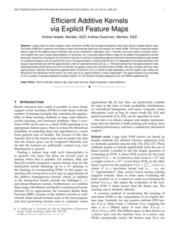
IEEE TRANSACTIONS ON PATTERN ANALYSIS AND MACHINE INTELLIGENCE, VOL. XX, NO. XX, JUNE 2011χ2(x,y), 0 x 1, y 9e 02χ2(x,y), 0 x 0.1, y 9e 030.250.0252.50.20.0220.150.015exactaddKPCAhom W 1 *hom W 1hom W rect *hom W dKPCAhom W 1 *hom W 1hom W rect *hom W rect0.060.040.020.60.8exactaddKPCAhom W 1 *hom W 1hom W rect *hom W rect0.0060.0040.0021000.020.04x0.0060.0080.01 3inters(x,y), 0 x 0.1, y 9e 031.40.40.002x0.0140.20xinters(x,y), 0 x 1, y 9e 020exactaddKPCAhom W 1 *hom W 1hom W rect *hom W rect10.140 3 2x 10 χ (x,y), 0 x 0.01, y 9e 041.5exactaddKPCAhom W 1 *hom W 1hom W rect *hom W rect0.01170.060.08x 10inters(x,y), 0 x 0.01, y 9e 04exactaddKPCAhom W 1 *hom W 1hom W rect *hom W rect0.60.40.20.1000.0020.004x0.0060.0080.01xFig. 2. Universal approximations. A useful property of the approximations (18) and (19) is universality. The figurecompares approximating the χ2 and intersection kernels kh (x, y) using features with n 3 components. From leftto right the dynamic range B of the data is set to B 1, 0.1, 0.01. The addKPCA approximation [1] is learned bysampling 100 points uniformly at random from the interval [0, 1], which tunes it to the case B 1. The homogeneousmaps are scale invariant, so no tuning (nor training) is required. Each panel plots kh (x, y) and the approximations forx [0, B] and y B/10. The figure also compares using a flat or rectangular window in the computation of (19). As averification, the homogeneous maps (19) are also derived as Nystrom’s approximations as explained in Sect. 3. Twothings are noteworthy: (i) addKPCA works only for the dynamic range for which it is tuned, while the homogeneousmaps yield exactly the same approximation for all the dynamic ranges; (ii) the rectangular window works better thanthe flat one in the computation of (19).Rectangular window. Consider now using a rectangularW (λ) rect(λ/Λ). The periodicization does not introduce any error: perΛ W K(λ) K(λ), for all λ Λ/2.Unfortunately, this window is not a PD, which maycause

The spectral analysis of the homogeneous kernels is based on the work of Hein and Bousquet [29], and is related to the spectral construction of Rahimi and Recht [7]. Contributions and overview. This work proposes a unified analysis of a large family of additive kernels, known as -homogeneous kernels. Such kernels are seen