Transcription
DEGREE PROJECT, IN OPTIMIZATION AND SYSTEMS THEORY , SECONDLEVELSTOCKHOLM, SWEDEN 2015Calibration of MultilaterationPositioning Systems via NonlinearOptimizationSEBASTIAN BREMBERGKTH ROYAL INSTITUTE OF TECHNOLOGYSCI SCHOOL OF ENGINEERING SCIENCES
Calibration of Multilateration PositioningSystems via Nonlinear OptimizationSEBASTIANBREMBERGMaster’s Thesis in Optimization and Systems Theory (30 ECTS credits)Master Programme in Applied and Computational Mathematics(120 credits)Royal Institute of Technology year 2015Supervisor at Ericsson: Daniel HenrikssonSupervisor at KTH: Johan KarlssonExaminer: Johan KarlssonTRITA-MAT-E 2015:62ISRN-KTH/MAT/E--15/62--SERoyal Institute of TechnologySCI School of Engineering SciencesKTH SCISE-100 44 Stockholm, SwedenURL: www.kth.se/sci
Kalibrering av System för MultilaterationsPositionerssystem genom Icke-linjär Optimering”SammanfattningI denna masteruppsats utvärderas en metod syftande till att förbättra noggrannheten i den funktion som positionerar sensorer i ett trådlöst transmissionsnätverk.Den positioneringsmetod som har legat till grund för analysen är TDOA (Time Difference of Arrival), en multilaterations-teknik som baseras på mätning av tidsskillnadenav en radiosignal från två rumsligt separerade och synkrona transmittorer till enmottagande sensor. Metoden syftar till att reducera positioneringsfel som orsakatsav att de ursprungliga positionsangivelserna varit felaktiga samt synkroniseringsfel i nätet. För rekalibrering av transmissionsnätet används redan kända sensorpositioner. Detta uppnås genom minimering av skillnaden mellan signalbaseradeTDOA-mätningar från systemet och uppskattade TDOA-mått vilka erhållits genomberäkningar av en given sensorposition baserat på optimering via en ickelinjärminstakvadratanpassning. Genom ett antal simuleringar testas sedan den föreslagnametoden med olika grundinställningar och olika grad av mätbrus samt ett varierande antal sensorer och transmittorer. Denna metod ger tydlig förbättring förestimering av systemparametrar och klarar även av att hantera multipla felkällorförutsatt att antalet mätningar är tillräckligt stort.2
AbstractThis master thesis presents an evaluation of a method for improving performanceof sensor positioning in a network of emitters. The positioning method used for theanalysis is Time Di erence of Arrival, TDOA, a multilateration technique based onmeasurements of di erences in signal travel time between a pair of synchronous andspatially separated pairs of emitters and a sensor. The method in question aims atreducing positioning errors caused by errors in initially reported emitter positionsas well as network synchronization errors by using already known sensor positionsto re-calibrate the network of emitters. This is done by minimizing the di erencebetween signal based TDOA measurements from the system and estimated TDOAmeasurements made by calculations based on given sensor positions by means ofnonlinear least squares optimization. Alterations of the method with di erentsettings and error contributions and with varying amount of sensors and emittersare tested throughout several simulations. The proposed method shows apparentresults of improving the system parameters and also copes well with contributingerrors provided that the amount of measurements is sufficiently large.
AcknowledgementsI would like to extend my greatest gratitude to Daniel Henriksson at Ericsson, who withhis knowledge and enthusiasm has given invaluable support and guidance throughoutthis project. I would also like to thank my supervisor at KTH, Johan Karlsson, who haswith his experience been a much appreciated support and dedicated advisor throughoutthe project.
Contents1 Introduction21.1Signal Based Positioning . . . . . . . . . . . . . . . . . . . . . . . . . . .21.2Thesis Outline . . . . . . . . . . . . . . . . . . . . . . . . . . . . . . . .32 Time Di erence of Arrival, TDOA42.1Method . . . . . . . . . . . . . . . . . . . . . . . . . . . . . . . . . . . .42.2Factors influencing accuracy . . . . . . . . . . . . . . . . . . . . . . . . .72.2.1Synchronisation errors and time delays . . . . . . . . . . . . . . .82.2.2Emitter position errors . . . . . . . . . . . . . . . . . . . . . . . .82.2.3Geometry . . . . . . . . . . . . . . . . . . . . . . . . . . . . . . .92.2.4Altitude . . . . . . . . . . . . . . . . . . . . . . . . . . . . . . . .92.2.5Multipath . . . . . . . . . . . . . . . . . . . . . . . . . . . . . . .103 Optimization and Method of Estimation113.1Unconstrained Optimization . . . . . . . . . . . . . . . . . . . . . . . . .113.2Nonlinear Least Squares . . . . . . . . . . . . . . . . . . . . . . . . . . .123.2.1Trust-Region-Reflective Least Squares Algorithm . . . . . . . . .123.2.2Nonlinear Least Square in Larger Scale . . . . . . . . . . . . . .143.2.3Weighted Nonlinear Least Squares Minimisation . . . . . . . . .15Cramér-Rao Lower Bound . . . . . . . . . . . . . . . . . . . . . . . . . .153.34 Modelling and Optimizing Antenna Position Errors in Cell Network4.119Formulation . . . . . . . . . . . . . . . . . . . . . . . . . . . . . . . . . .204.1.1System of Insufficient Rank . . . . . . . . . . . . . . . . . . . . .214.2Determination of Weights . . . . . . . . . . . . . . . . . . . . . . . . . .224.3Cramér Rao Lower Bound Analysis . . . . . . . . . . . . . . . . . . . . .235 Simulations5.126Method . . . . . . . . . . . . . . . . . . . . . . . . . . . . . . . . . . . .6 Results286.0.1Weighted and Non-Weighted Least Squares . . . . . . . . . . . .286.0.2No error in sensor positions . . . . . . . . . . . . . . . . . . . . .296.0.3Small error in sensor positions . . . . . . . . . . . . . . . . . . .306.0.4Large error in sensor positions . . . . . . . . . . . . . . . . . . .317 Discussion7.12632Future work . . . . . . . . . . . . . . . . . . . . . . . . . . . . . . . . . .533
8 Conclusion35Appendix A TDOA Positioning of Sensors36A.1 TDOA Positioning by Sum of Least SquaresAppendix B Positioning with height parameter. . . . . . . . . . . . . . .3637
GlossaryTDOATime Di erence of ArrivalETDOAExpected Time Di erence of ArrivalGPSGlobal Positioning SystemNLLSNonlinear Least SquaresTTFFTime to First FixTOATime of ArrivalCRLBCramér-Rao Lower BoundGDOPGeometric Dilution of PrecisionFIMFischer Information MatrixNomenclatureeEmitter positioneestEstimated emitter positionsSensor positionsestEstimated sensor positions̃Estimated sensor positiongEmitter position error TDOA Measurement noiseTime synchronization delay TDOA value1
1IntroductionThis aim of this thesis is to evaluate an algorithm for improving positioning accuracy inwireless networks. Primarily, aspects of improving Time Di erence of Arrival (TDOA)positioning are considered. However, some of the methods used are also applicable toother positioning methods in wireless networks and other similar signal based positioningmethods. More specifically, the algorithm to be evaluated will address certain commonerror contributions to see whether an adjusting calibration can decrease systematicalerrors and their impact on positioning accuracy.1.1Signal Based PositioningThere are many examples of wireless and signal based systems that feature the possibility of locating the position of an emitting or receiving unit. Global Positioning System,GPS, is a widely adopted positioning method using several time synchronized satellitesmaking signal time measurements and multilateration to locate a receiving GPS signalunit [1].It has become increasingly important to be able to position a mobile device accurately in a cellular network. Positioning a mobile device in a mobile network can ,e.g.,enable localization of emergency calls, advanced location based services and possiblealso aid network traffic optimization [2]. As mobile network coverage is increasing andthe technology is becoming increasingly advanced, the methods of positioning are underconstant improvement [2].Both GPS positioning methods and cellular network positioning methods are based onmeasurements on signals from distant satellites and antennas respectively. An obstaclefree environment, where signals can travel without disturbance between the transmittingand receiving unit is to be preferred, however that is in most environments of application not possible. For example, these disturbances lead to multipath errors which willbe described further in Section 2.2. These methods are not ideal for ,e.g., urban andindoor environments. A more recent and evolving positioning feature is that of locatingunits with local wireless networks, such as WiFi or Wireless Sensor Networks, WSN[4][5]. An example of application is indoor robot localisation, as described by Cheng etal. [4].2
As the computational capacity of network related equipment increases, it is possible tocombine several positioning methods to increase accuracy. These are known as HybridPositioning systems. By combining results from multiple positioning methods, knowingthe limitations and sources of errors for each method, it is possible to achieve a higheraccuracy than when applying one single method [7]. A common method of combiningdi erent methods is for a GPS to achieve assistance data from a cellular networks toimprove start up speed and decrease the Time-to-First-Fix, TTFF, known as the timerequired for a GPS receiver to acquire necessary GPS signals and fix a first position [7].The assistance date sent from the cellular network could for example be in what cellsector the unit is situated whereby the GPS can limit its scope of search significantly [7].The above mentioned positioning methods are examples of methods using known information from emitters to locate unknown positions of sensors. However, the oppositecan also be true. An example is when trying to locate from where radar signals are sentfrom. By measuring the signal and their characteristics from di erent known locations itis possible to estimate where the signals are transmitted from [6] [3]. One such methodis known as Passive Radar Localization where positioning by means of TDOA is oneof the most fundamental and popular localization methods [6]. This method will bedescribed in more detail later in this thesis. However, the emphasis in this thesis willbe on sensor positioning in a network of emitters.1.2Thesis OutlineThe proposed method aims to improve accuracy of a TDOA sensor positioning systemprone to systematic errors. More specifically the algorithm addresses errors caused byfaulty position information and time synchronization errors in the positioning network.The general idea is to use already known sensor positions to refine emitter system parameters and synchronization.What will follow is an introduction to TDOA positioning including general theory anda description of common error contributions and how these a ect accuracy. Thereafter,the proposed method and alterations of it will be described. A description of the optimization algorithms used are presented followed by a simulations results from testingthe proposed method with di erent settings and parameters.This thesis aims at evaluating the proposed method to see whether it proves to beefficient in increasing the accuracy in a positioning network. The method is evaluatedthrough a theoretical model and if the method proves to be successful, the thesis can beused as a foundation when implementing in a physical network.3
2Time Di erence of Arrival, TDOAThere are numerous methods of estimating a stationary sensor position from measurements on for example signal arrival times, angle of arrival and Doppler shifts ofelectromagnetic waves at di erent sites [11]. This thesis focuses on multilateration,a hyperbolic location system, more commonly known as Time Di erence of Arrival(TDOA), which exploits the di erence in arrival time between transmitted signal fromemitters to a sensor that is to be positioned. TDOA is not to be confused with Time ofArrival (TOA), a trilateration positioning method. TOA measures the absolute time ittakes for the signal to travel from the emitters to the sensor. When measuring TOA itis important that both the emitters and the sensors are time synchronized. If they arenot synchronized, TDOA is to prefer, eliminating such errors [12].2.1MethodLet s 2 Rd be a sensor position and ej 2 Rd , j 1, 2, 3, be the positions of threeemitters. These emitters are synchronized and the sensor which is to be positionedreceives a signal from each of these emitters. The sensor calculates the TDOA foreach unique pair of emitters 12 , 13 , 23 . Each TDOA measurement corresponds to anequation: ij sei sej (1)where k·k denotes the euclidean distance in Rd .In the two dimensional case, at least three emitters are needed to locate a sensor. Togive a simple example let us look at a situation with two emitters and one sensor. Lete1 ( D/2, 0) and e2 (D/2, 0) and s (x, y). The measured TDOA values for thepair of emitters are given by:qpy 2 (x D/2)2qp4t2 ks e2 k (x e2,x )2 (y e2,y ) y 2 (x D/2)2 p p 12 4t1 4t2 y 2 (x D/2)2y 2 (x D/2)2 .4t1 kse1 k (xe1,x )2 (ye1,y ) (2)The last equation can also be written asx22 /4 12y2 1. 12 )/4(D24(3)
This can be recognized as a hyperbolic equation where the solution has asymptotes alongy sD2 12 )/4x.2 /4 12(4)The solution to the equation corresponds to the sensor being somewhere along a hyperbola as can be seen in Figure 1 for di erent values of 12 .3210τ 0.4τ 0.8τ 1.2τ 1.4-1-2-3-3-2-10123Figure 1: Hyperbolas as a result of di erent TDOA measurementsThe measurements made in the systems are prone to errors. Each TDOA measurementhas an uncertainty ij and stated as: ij ksei kksej k ij1 i j n.(5)This results in each hyperbola including a margin of error as can be seen in Figure 2.The hyperbolas are then better described as hyperbolic areas.3210-1-2-3-3-2-10123Figure 2: TDOA measurement with an uncertainty relating to measurement noise5
With three emitters there is a set of three TDOA values: 12 se1 se2 12 13 se1 se3 13 23 se2 se3 23 .(6)To locate s we will want to solve the following system of equations for the unknownvariable sest , the estimated position of s: seste1 seste2 12 12 0 se1 se3 13 13 0e2 se3 23 23 0. sestestestest(7)The three equations in (7) correspond to three hyperbolic areas with a certain widthcorresponding to the uncertainty in the measurements, as seen in Figure 3. One expects to find the sensor in question where these hyperbolas intersect.x.xxFigure 3With m available emitters there will be a total of K TDOA measurements and equationswhere K is given by all pairwise unique enumerations of emitters mm(m 1)K .22(8)If we disregard any measurement noise, the problem will be to solve an over determinedsystem when md 1 where d once again is dimensions of the space in which thepositions that are to be determined. However in the presence of measurement noise,the hyperbolas will almost certainly intersect in several di erent points. The results isan estimation problem where one seeks to find the most probably solution. There is alarge amount of research in finding as accurate and efficient methods of solving theseestimation problems (e.g. [19][20][21]). In this thesis a non-linear least squares method6
will be implemented, similar to what is done in [12]. In short one then defines F (sest )to be a vectorized function consisting of all equations corresponding to each TDOAmeasurement v 1, 2, ., Kfv (sest ) sestej sestek jk jkfor 1 j k m.(9)The estimation is formulated as an minimization of the sum of least squares. Moredetails of how to find the optimal values are found in Section 3. In the evaluation of theproposed method in this thesis a TDOA sensor positioning model is used as a source ofreference and comparison. Please refer to Appendix A for more details.2.2Factors influencing accuracyIn addition to the signal measurement noise there are numerous other factors that a ectthe accuracy of TDOA positioning. Below are some examples such of factors of whichsome will be addressed further in this thesis. Synchronisation errors and time delays Emitter position errors Geometry Altitude -40-20020406080100Figure 4: Sensor and emitters of a TDOA measurement7
2.2.1Synchronisation errors and time delaysIf the emitters are not perfectly time-synchronized or if there are signal path time delays,the measured distance time values will contain errors that will a ect the accuracy. Anexample of how synchronisation errors a ect the positioning of a sensor in a emitternetwork is shown in Figure 5. The sensor is positioned in the middle of three emittersas shown in Figure 4 and one of the emitters is given a time delay.8Sensor Positioning Error76543210-5-4-3-2-101Time Delay of one emitter [s]2345 10 -8Figure 5: Sensor positioning error with unknown time delayIf we know for a fact that the two emitters have perfect synchronization it can be thecase that one, or both, signals sent from the two emitters are subject to path delays. Theemitters are said to emit the signals at a certain time, t, however the signals are for somereason, delayed and actually can be considered sent out a slightly later, t 4t. Thiscould for example be caused by obstacles in the environment. This in combination withsynchronization errors will have a considerable impact on the accuracy and a method ofreducing these contributions will be addressed in the proposed method.2.2.2Emitter position errorsWhen estimating positions from TDOA measurements it is of great importance to haveaccurate emitter positions in the system. When building a wireless network that is tobe used for positioning of sensors, each emitter position is determined and noted in thesystem. It is in some cases difficult to be precise when determining these positions andoften it is a time consuming process to achieve high accuracy. These positions have asignificant role in the estimation of sensor positions and if the actual emitter positionsdi er from the positions known to the system a systematic error in positioning accuracywill be apparent [13]. An example of how errors in given emitter positions a ect thepositioning of a mobile unit in a mobile network is shown in Figure 6. The sensor isonce again located in the middle of three emitters as shown in Figure 4 and Figure 68
Maximum Sensor Positioning Error [m]12108642002468101214161820Emitter displacement [m]Figure 6: Sensor positioning error with emitter position errorsshows the maximum positioning error when one of the emitters actual positions di ersfrom the known position to the system.2.2.3GeometryThe geometry of where the measurements are taken have an impact on the accuracy.Figure 7 shows an example of how the geometric dilution a ects the estimation whenthe sensor is moved further way from a pair of emitters. As can be seen, the area ofuncertainty increases when the sensor is placed further away from the two emitters.xxx.x.Figure 7: Example of Geometric DilutionA common method of analyzing to what extent is the geometry a ects is to look at theGeometrical Dilution of Precision, GDOP. The GDOP is a result of The Cramér-RaoLower bound, CRLB, which is a well known result of mathematical statistics. It givesa lower bound of the covariance of estimated parameters. For more information on theCramér-Rao Lower bound is found in Section 3.3.2.2.4AltitudeFor this thesis, the focus is on horizontal sensor positioning in two dimensions. Howeverit is possible that the emitters and sensors have vertical components. This will havean impact if disregarded in the estimation problem. Figure 8 illustrates the maximumposition error when the vertical component is disregarded in the calculations. Once9
again, we have the same setup as in Figure 4. If one of the emitters were to have an vertical component, h, and the sensor having zero vertical component then the maximumpositioning error is shown in Figure 8.As mentioned previously, the evaluation made in this thesis will regard a two-dimensionalsetting although the theory is applicable in general dimension. However, in Section Bpresents some short results on how height a ects the proposed method.Figure 8: Sensor positioning error when disregarding height parameter2.2.5MultipathWhen signals propagate between an emitter and a sensor it is often the case that thereare obstacles in the environment. The signal measurements are made on nonline-ofsight paths which will di er from the line-of-sight signal travel distance [10]. Theseerrors generally have a large contribution to the overall accuracy and are especiallyprominent in indoor settings. To dampen the magnitude of this error contribution, thereceiver of the di erent signals searches for the signal for the signal which has travelledthe shortest time. This signal is likely to give the most accurate measurement [10].10
3Optimization and Method of EstimationWhat follows is an introduction to the optimization method used for the analysis ofthe proposed method and the algorithm behind Matlab’s solver lsqnonlin, later used inthe simulations. This is followed by theory concerning estimation and the Cramér-RaoLower Bound.3.1Unconstrained OptimizationWe will be interested in minimizing a function where no constraints are placed on thevariables. This is known as unconstrained optimization and what follows is generaltheory of optimality conditions concerning unconstrained optimization. Let y(x) be afunction of the variables x (x1 , ., xn ) that we wish to minimize,minxy(x).(10)To define optimality conditions we denote x to be a possible solution to the problem.A global optimum to (10) is a point x for whichy(x ) y(x) for all x,(11)whereas a local optimum is a point x for whichy(x ) y(x) for all x such that kxx k ,(12),for some 0 [25]. For unconstrained problems it is very difficult or impossible toevaluate global optimality. In general, to determine a global optimum, one needs information about the function in question for each and every point. The algorithms usedto solve these types of problems only has information about a finite set of points of thefunction. However it is possible to state conditions for local optimality [25].Consider the Taylor series expansion of y around the point x :1y(x p) y(x ) 5y(x )T p pT 52 y( )p(13)2where is a point between x and x and p is a nonzero vector. Suppose that x is alocal optimum then there are no feasible descent directions from this point. This meansthat the gradient at this point must be zero [25],5 y(x ) 0.11(14)
This is known as the first-order necessary condition for a local minimum [25]. Howeverthis condition is not enough to state the point being a local minimum. To be furtherconfirm that a point is local minimum we need to look at the second derivatives. Considerthe Taylor series expansion for a point for which the first-order necessary condition issatisfied (5y(x ) 0):1y(x p) y(x ) pT 52 y( )p.(15)2The second-order necessary condition states that 52 y(x ) must be positive semidefinite. If it is not semidefinite then bT 52 y(x )b 0 for some b. This also means thatbT 52 y( )b 0 if k x k is sufficiently small. Thus, if p is chosen as a small multipleof b, the point will be a close approximate to x such that by the Taylor expansion itcan be concluded that y(x) y(x ) [25], which is a contradiction.Furthermore, there is a second-order sufficient condition. A condition that is sufficientto ensure a local minimum and consists of the first-order necessary condition togetherwhith the condition that 52 y(x ) is positive definite. Such an x is known as a strictminimizer [25].3.2Nonlinear Least SquaresThe model evaluated in this thesis will involve fitting a set of variables to a large numberof data points. Because of measurement noise and other contributing errors it can notbe expected that it is possible to find an exact solution. We instead want to find ansolution that fits to the collected data by means of reducing the residual error. Let F (x)be a vector-valued function with Fv fv (x). Each fv (x) is a function of the residualof data point v 1, ., n and x is a vector of variables. The nonlinear least squares,NLLS, problem is then defined as:minxXfv2 (x) minxvkF (x)k22 .(16)A simple yet powerful method of solving (16), is a method based on trust regions. It is aniterative method that searches for points that fulfill second-order necessary condition ofa local optimum. In this section follows a description of the method used and underlyingtheory.3.2.1Trust-Region-Reflective Least Squares AlgorithmConsider a scalar valued nonlinear function f (x), with vector arguments x, that issubject to minimization. Let x0 be an initial point and one wishes to move from this12
point to decrease the current function value. The idea is to, in the neighbourhood N ofx, approximate f with a more simple function q. The neighbourhood, N , for which q isa sufficiently good approximation of f is called the trust region. A step, s, is calculatedby minimizing q(s) over N ,min {q(s), s 2 N } .xIf f (x0 s) f (x0 ), the initial point is updated, x0 s. If f (x0 s)(17)f (x0 ), x0remains unchanged and the trust region N is reduced in size after which the process isrepeated. The key aspects of a trust-region optimization is choosing how to approximatethe function, how to choose and alter the size of the trust region N and how to bestsolve the subproblem.A standard trust-region method is described in [14]. The idea is to approximate f byletting q be defined as the first two terms of the Taylor expansion of f . The subproblemis thus stated as:mins 1 Ts Hs sT g such that k Dsk 22 4 .2(18)where H is the Hessian and g is the gradient of f at x, D is scaling matrix with diagonal entries and 4 a positive scalar. There are a good number of algorithms for solving(18) and many of these are mentioned in [14]. However these algorithms require timethat is proportional to several factorizations of the Hessian, H, which becomes costlyprocess [16][17]. In trust-region algorithms the most computationally costly process isto evaluate a step at the current iterate [15]. The algorithm used in this thesis is theso called ”Indefinite Dogleg Algorithm” first described in by Schultz et. al. [18] andlater evaluated and analyzed by Byrd et al [15] and Branch et. al. [16]. It makes adi erent approach to approximating (18) by restricting the trust-region subproblem toa subspace S in two dimensions. By choosing two suitable directions to span a space Sit is possible to with high accuracy and good convergence optimize a function f 2 Rn[15].To explain the di erence from and the computational advantages of the used InfiniteDogleg Algorithm, what follows is an introduction to important aspects of algorithmsused to solve (18). One such important concept is the so called -optimality. -optimalmethods take steps which are at least a fraction of the true optimal value. We definea more formal formulation of -optimality by the following definitions:Definition 1 (Step function). The function q is called a step function if: Rn Rn n (0, inf) ! Rn . Here denoted as q(g, H, 4) .13
Definition 2 (Optimal step computing function). For any g 2 Rn , H 2 Rn n and4 0. We denote the solution to (18) to be q (g, H, 4). An optimal step computingfunction is thus refered to as q .Definition 3. For q 2 Rn , let pred(q, g, H) qT g1 T2 q Hq.Definition 4 ( -Optimal). For 2 (0, 1], a step computing function q is if for any symmetric H 2 Rpred(q(s, H, 4), s, H)nxnoptimaln, s 2 R , and 4 0: pred(q (s, H, 4), s, H).Byrd et al. [22] show that if a trust-region step function satisfies three conditions it hasthe same global and local convergence as a -optimal step computing function. However,the conditions presented below are compared to -optimality somewhat weaker [22].1. There are c1 , c 1 such that for all 4 0, s 2 Rn and H 2 Rnxn .kskc1 ksk min{4, c 1 kHk}.pred(q(s, H, 4), s, H)2. Letbe the smallest eigenvalue of H. There is a c2 0 s.t. for all s 2 Rn , 4 0and H 2 Rn npred(q(s, H, 4), s, H)3. IfH1c2 ((H))42 .s 4 and H 2 Rn n is positive definite, then q(g, H, 4) H1s.The proposed ”Indefinite Dogleg Step Computing Function” satisfies the above conditions.The subspace S is spanned by s1 and s2 where s1 is the direction of the gradient, g,and s2 is defined to be an approximate Newton direction or, if the Hessian is indefinite,a direction of negative curvature.s2 8 H · s2 g if H positive definite: sT · H · s2 0 if H indefinite.2(19)With these vectors one aims to encourage global convergence with steepest descent ornegative curvature direction and also enable local convergence with the Newton stepwhen possible. For more details about this algorithm see Schultz. et al. [18].3.2.2Nonlinear Least Square in Larger ScaleThe solver used in the simulations is lsqnonlin implemented in Matlab which solves nonlinear least squares using Trust-Region-Reflective Least Squares Algorithm as describedin the previous section. However, when the system increases in size, the solver in Matlabmakes an adjustment to the algorithm to improve efficiency. To avoid finding secondderivatives of all f (x) an approximate Gauss Newton direction is found instead to definethe subspace S. Let J be the Jacobian of F (x). s is found by solvingmin Js F 22 .14(20)
The method of preconditioned conjugate gradients is used in every iteration to find anapproximate solution to the normal equations [24].3.2.3Weighted Nonlinear Least Squares MinimisationA small error in supplied information to an optimization model can, due to the formulation of the equations and the optimization, have a significant impact on t
av en radiosignal fr an tv a rumsligt separerade och synkrona transmittorer till en mottagande sensor. Metoden syftar till att reducera positioneringsfel som orsakats av att de ursprungliga positionsangivelserna varit felaktiga samt synkroniserings-fel i na tet. F or rekalibrering av transmissionsna tet anva nds redan ka nda sensor .