Transcription
Konrad Zuse’s Rechnender Raum(Calculating Space)1st. re-edition1 written in LATEX by A. German and H. ZenilAs published in A Computable Universe: Understanding & ExploringNature as Computation, World Scientific, 2012Painting by Konrad Zuse (under the pseudonym “Kuno See”).Followed by an Afterwordby Adrian German and Hector Zenil12with kind permission by all parties involved, including MIT and Zuse’s family.The views expressed in the afterword do not represent the views of those organisationswith which the authors are affiliated.21
Calculating Space (“Rechnender Raum”)‡Konrad ZuseContents1 INTRODUCTION12 INTRODUCTORY OBSERVATIONS2.1 Concerning the Theory of Automatons . . . . . . . . . . . . .2.2 About Computers . . . . . . . . . . . . . . . . . . . . . . . . .2.3 Differential Equations from the Point of View of the Automaton Theory . . . . . . . . . . . . . . . . . . . . . . . . . . . .2.4 Maxwell Equations . . . . . . . . . . . . . . . . . . . . . . . .2.5 An Idea about Gravitation . . . . . . . . . . . . . . . . . . . .2.6 Differential Equations and Difference Equations, Digitalization2.7 Automaton Theory Observations of Physical Theories . . . .3358101313143 EXAMPLES OF DIGITAL TREATMENTAND PARTICLES3.1 The Expression “Digital Particle” . . . . . . . .3.2 Two-Dimensional Systems . . . . . . . . . . . .3.3 Digital Particles in Two-Dimensional Space . .3.4 Concerning Three-Dimensional Systems . . . .1919273034OF FIELDS.4 GENERAL CONSIDERATIONS374.1 Cellular Automatons . . . . . . . . . . . . . . . . . . . . . . . 374.2 Digital Particles and Cellular Automatons . . . . . . . . . . . 394.3 On the Theory of Relativity . . . . . . . . . . . . . . . . . . . 39‡Schriften zur Datenverarbeitung, Vol. 1, 1969 Friedrich Vieweg & Sohn, Braunschweig, 74 pp. MIT Technical TranslationTranslated for Massachusetts Institute of Technology, Project MAC, by: Aztec School of Languages, Inc., Research Translation Division(164), Maynard, Massachusetts and McLean, Virginia AZT-70-164-GEMIT MassachusettsInstitute of Technology, Project MAC, Cambridge, Massachusetts 02139—February 19702
4.44.54.64.7Considerations of Information TheoryAbout Determination and Causality .On Probability . . . . . . . . . . . . .Representation of Intensity . . . . . .5 CONCLUSIONS.4148525355
DEDICATION TO DR. SCHUFFThe work which follows stands somewhat outside the presently acceptedmethod of approach, and it was for this reason rather difficult to find a publisher ready to undertake publication of such a work. For this reason I amindebted to the Vieweg Press and especially to Dr. Schuff for undertakingpublication. Dr. Schuff suggested that a summary be printed in the Journal “Elektronische Datenverarbeitung” (Electronic Data Processing), whichappeared last year.The tragic death of Dr. Schuff has deeply shaken his friends, and we willalways remember him with affection.
1INTRODUCTIONIt is obvious to us today that numerical calculations can be successfully employed in order to illuminate physical relationships. Thereby we obtain amore or less close interrelationship between the mathematicians, the physicists and the information processing specialists, corresponding to Fig. 1.Mathematical systems serve for the construction of physical models, thenumerical calculation of which is carried out today with electronic data processing equipment.The function of thedata processing specialists is primarily that offinding the most useful numerical solutionsfor the models whichthe mathematicians andphysicists have developed. The feedback effect of data processingon the models and thephysical theories itself isexpressed indirectly inthe preferential use ofthose methods for whichnumerical solutions areparticularly easy to obtain.The close interplaybetween the mathematicians and the physicistshas had a particularlyfavorable effect on theFigure 1development of modelsin theoretical physics. The modern quantum theory system is very largelypure and applied mathematics. The question therefore appears justifiedwhether data processing can have no more than an effectuating part in theinterplay or whether it can also be the source of fruitful ideas which themselves influence the physical theories. The question is all the more justifiedsince a new branch of science, automaton theory, has developed in closecooperation with data processing.1
In the following pages, several ideas along these lines will be developed.No claim is made to completeness in the treatment of the subject.Such a process of influence can issue from two directions:1. The development and supplying of algorithmic methods, which canserve the physicist as new tools by which he can translate his theoretical knowledge into practical results. Among these are included firstall numerical methods, which are still the primary tool in the use ofelectronic calculating machines. The ideas expressed in the chapterswhich follow could contribute particularly to the problem of numericalstability.Among these are symbolic calculations, which command an ever growing importance today. The numerical calculation of a formula is notmeant by this, but the algebraic treatment of the formulas themselvesas they are expressed in symbols. Precisely in quantum mechanics, extensive formula development is necessary before the actual numericalcalculation can be carried out. This very interesting field will not becovered in the material which follows.2. A direct process of influencing, particularly by the thought patternsof automaton theory, the physical theories themselves could be postulated. This subject is without a doubt the more difficult, but also themore interesting.Therein lies the understandable difficulty that different fields of knowledge must be brought into association with one another. Already the fieldof physics is splitting up into specialized areas. The mathematical methodsof modern physics alone are no longer familiar to every mathematician andan understanding of them requires years of specialized study.But even the theories and fields of knowledge related to data processingare already dividing into different special branches. Formal logic, informationtheory, automaton theory and the theory of formula language may be citedas examples. The idea of collecting these fields (to the extent which they arerelevant) under the term “cybernetics” has not yet become widely accepted.The conception of cybernetics as a bridge between the sciences is very fruitful,entirely independent of the different definitions of the term itself.The author has developed several basic ideas toward this end, which heconsiders of value to be presented for discussion. Some of these ideas intheir present, still immature form may not be reconcilable with the provenconcepts of theoretical physics. The goal has been reached if only discussion2
occurs and provokes stimulation which one day leads to solutions, which arealso acceptable to the physicists.The method applied below is at present still heuristic in nature. Theauthor considers the conditions not yet ripe for the formulation of a precise theoretical system. First of all, the existing mathematical and physicalmodels will be considered in Chapter 2 from the viewpoint of the theory ofautomatons. Several examples of digital models are presented in Chapter 3,and the expression “digital particle” is introduced. In Chapter 4, severalgeneral thoughts and considerations based on the results of Chapters 2 and3 will be developed, and in Chapter 5, the prospects for the possibility offurther developments are considered briefly.22.1INTRODUCTORY OBSERVATIONSConcerning the Theory of AutomatonsThe theory of automatons today is already a widely developed, and to anextent very abstract, theory about which considerable literature has beenwritten. Nevertheless, the author would like to distinguish between the actual automaton theory itself and the thought patterns connected with thistheory, of which considerable use will be made in the following chapters.A thorough understanding of the automaton theory is not necessary to anunderstanding of the chapters which follow.The automaton theory appeared at about the same time as the development of modern data processing equipment. The design and the workingmethod of these arrangements necessitated theoretical investigations basedon different mathematical methods; for example, that of mathematical logic.The first useful result of this development was connection mathematics, inwhich particularly the statement calculus of mathematical logic can play animportant part. Of particular importance is the realization that all information can be broken up into yes-no values (bits). The “truth values” ofstatement calculus assume only two ratings (true and false). The connectingoperations and the rules of statement calculus can therefore be viewed as theelementary operations of information processing. Fig. 2 shows the elementary connections corresponding to the three basic operations of statementcalculus, conjunction, disjunction and negation.Further research led to introduction of the term “state” of an automaton.In addition, input data and output data play a role. From input and initialstate the new state and the output are obtained, corresponding to the algorithm built into the automaton. Fig. 3 shows the schematic diagram of an3
Figure 2Figure 3automaton for a two-place binary register. In the figure, E1 and E0 representthe inputs on which a two place binary number can be entered and A2 , A1and A0 represent the outputs, which have the meaning of a three-place binary number. The two-place binary number formed from the figures A1 andA0 is relayed back to the automaton and represents the eventual state of thebinary number. (In this case the states symbolize a number already enteredinto the addition process, to which the number E1 , E0 is to be added).The algorithm given by the automatoncan be represented by state tables in simplecases. These have the form of a matrix, andfor every state and every input combinationthey give the resultant state or output combination. Fig. 4 shows the state table forthe automaton in Fig. 3. In this particularcase the state table represents an additiontable. The theory of the automaton investigates the different possible diffractions ofsuch an automaton and sets forth a series ofFigure 4general rules concerning its method of operation. It is important for what follows that the terms finite, autonomous andcellular automaton be understood. A finite automaton works with a discretenumber of discrete states; it is roughly equivalent to a digital data processingmachine, which is made up of a limited number of elements, each elementcapable of taking a limited number of states (at least two), with the resultthat the whole automaton can accept only a limited number of states. Similar conditions hold for the inputs and outputs. The autonomous automatoncan accept no inputs (the outputs are also relatively inconsequential). It can4
be represented, therefore, by a machine that operates independently, oncestarted. Its states follow linearly in sequence, once the initial combinationhas been started, and the operational process cannot be influenced externallyby the absence of one of the inputs.The cellular automaton represents a special form of automaton built outof interrelated, periodically-recurring cells. This type of automaton is ofparticular importance for the observations which follow. Later it will bediscussed in greater detail.By the term “automaton theoretical way of thinking” we understand amanner of observation according to which a technical, mathematical or physical model is viewed from the standpoint of a lapse of states, which followone another according to predetermined rules.2.2About ComputersThe automaton theory can be used as an abstract mathematical system,yet these thought structures can also be related to technical models, andsimilarly the automaton theory can be used for describing automatons, particularly those suited for information processing. In current expanded usage,the term “compute” is identical with “information processing.” By analogy,the terms “computer” and “information-processing machine” may be takenas identical.We distinguish between two classes of computers: analog computers anddigital computers. In an analog computer, the steps in the calculation areperformed in an “analog” model. Magnitudes representing numerical valuesare theoretically represented through continual physical magnitudes, such aspositions of mechanical parts (torsion angle), tension, velocities, and the like.The machine operates essentially without end. The represented values lieobviously below certain technical limits. These are established by maximumvalues and by the accuracy of the system. The maximum values are given bya clearly-defined upper limit which corresponds to the technical limits of thesystem. In contrast, the accuracy has no clearly-defined magnitude, becauseit depends on change and on external influences (temperature, moisture,the presence of disturbing fields, etc.) One well-known analog computer isthe slide rule. Fig. 5 shows a mechanical adding mechanism the form ofa lever which can be replaced with a rotating mechanism with gears, as inFig. 6. This mechanism is known in engineering by the inappropriate term“differential mechanism” and is employed in the rear axle of every automobile.A typical construction element of analog machines is represented by theintegration mechanism shown in Fig. 7. This operates with a friction disc A5
Figure 5Figure 6in contact with a friction wheel B. The distance r of the friction wheel Bfrom the axle of A can be varied. In this way, the mechanism can be usedfor integration. In modern analog instruments, these mechanical elementsare replaced by electronic ones. An integration can, for example, be carriedout by charging a condenser.Noncontinuous processesare generally not reproducible with analog instruments; in other words, analog computers are poorly designed for these processes.With digital computers,all values are represented bynumbers. Because a digiFigure 7tal computer can hold onlya certain limited sum of numbers, there is available for the representation ofcontinuous values only a limited supply of values. This implies considerabledivergence from mathematical models. Mathematical values are subject tothe concept of infinity in two respects.First, the absolute magnitude of the numbers is unlimited; furthermore,between any two given values an infinite number of intermediate values maybe assumed to exist. For this reason, computers have (independent of thenumber code employed) maximum values which, out of technical considerations (number of places of the register and storage), cannot be exceeded.In addition, the values proceed in step-fashion. There are neighboring values between which no additional intermediate values may be inserted. This6
results in limited accuracy among other consequences. In contrast to theanalog computers, the accuracy of digital computers is strictly defined andis not subject to any coincidental influences.A further conclusion is that no digital computer can precisely reproducethe results of processes defined by arithmetic axiom. Thus, for example, themathematical formulaa·b bahas general validity, with the one exception that a cannot be equal to 0.There is no finite automaton capable of reproducing this fact precisely andgenerally. It is possible, nevertheless, by increasing the number of places before and after the decimal point, for a digital computer to approach infinitelyclose to the laws of arithmetic.We in the field of mathematics have already become so accustomed to theconcept of infinity that we accept it without considering that every infiniteterm is related to a series expansion or to a limiting process (“for everynumber there is one which follows it”). By relating this process to automatontheory, we obtain in place of a static, predetermined, finite automaton a seriesof automatons which are constructed according to a definite plan and differfrom one another only in the number of places. The plan for constructionof an automaton with n places is given; in addition, there are instructionsfor converting an n-place automaton to one with n 1 places. By use of thelimiting process limn with the aid of series expansion the automaton rulefor arithmetic operations is obtained.The digital computer, because of its special ability to handle not onlynumbers but also general information (in contrast to the analog computer),has opened up completely new fields, discussed below in greater detail. Ingeneral, all calculation problems can be solved on a digital computer, whereasanalog computers are better suited to special tasks. It must be stressed thatdigital computers work in a strictly determinative way. Using the samealgorithm (i.e., the same program) and introducing the same input values,the same results must always be obtained. The limited accuracy alwaysresults in the same degree of inaccuracy in the results when an operation isperformed several times on the same inputs. This is in contrast to the analogcomputer, in which the limited accuracy has a different effect each time theprogram is run and can be expressed only in terms of statistical probability.By way of supplementary comments, it may be observed that hybridsystems have been developed which consist of a mixture of the principles ofthe digital and of the analog computer.7
This can be simply carried out v ia a system inwhich the two computers operate side-by-side. They arejoined by a digital-analogconverter and an analogdigital converter (Fig. 8). InFigure 8systems of this type, the single parts of the problem are divided in such a way that the more appropriatedevice is chosen for each subdivision of the problem.The joining of the two systems can also beaccomplished by the representation of the values themselves. Thus, for example, a magnitude may be characterized by the pulse density (Fig. 9). Pulses themselves have a digitalcharacter, for they are normalized in intensityFigure 9and duration; they are therefore digital, buttheir density (the number of pulses per unit time) can have any number ofintermediate values, and it is therefore analog in character. A commonly-heldopinion today is that the human nervous system operates on this principle.2.3Differential Equations from the Point of View of the Automaton TheoryObservation of several differential equations reveals that this way of thinkingis by no means self-evident to mathematicians and physicists. There are atour disposal a number of models of physical data, which can be representedby differential equations. For example, we can take a simple differentialequation to represent the upper surface shape of a liquid in a rotating vessel, according to which at every point on the surface, the normal to thesurface is determined by the vector sum of the gravitational and centrifugalaccelerations (Fig. 10).This equation is written:rω 2y0 gwhere ω is the angular velocity of the container.The solution is very easy to obtain analytically:y ω2 2·r2g8
In reality, we have here an expression valid for the situation onlyafter equilibrium has been established. For every equilibrium situation there is an initiating action.In the experiment with a rotatingvessel initially at rest, the rotatory motion must be transferred tothe liquid through frictional forces.Figure 10Only after complex wave interaction, which diminishes with time, will equilibrium be established. For thisreason it is not possible to describe the actual processes in this transition bymeans of our differential equation. The processes taking place during thisperiod are considerably more complicated, and they are almost impossibleto describe mathematically. We realize also that it is not necessary to followeach of these complicated processes when only the final state is of interestto us.The relationships are very similar to many partial differential equations.These equations are used to describe the stress divisions of an equilibriumsituation in plane and solid stress states. The establishment of equilibriumoccurs in actuality v ia a highly complicated sequence of steps, in whichonce again the braking of these processes is the condition for the eventualestablishment of equilibrium.Differential equations describe only the final condition in the case ofthe theory of ideally incompressible fluids. The actual process leading toestablishment of the end condition of equilibrium from a state of rest ishardly conceivable without taking compressibility and braking processes intoaccount.In the case of these differential equations, the issue is not one of a fundamental law, which can be described in terms of automaton theory as afunctional variable of different, sequentially-occurring states. This also hasan influence on the possible numerical solutions. Differential equations whichdescribe an allowed sequence of states of a system are often easier to solvenumerically than those which represent no more than a control function overthe final state. In fact, solutions for such end states must usually be foundin a stepwise solution, often with help of a relaxation process. It is not necessary to attach value to the step-wise approximations of the final state inorder to simulate natural or technical processes; thus, it is possible to applymathematically-simpler processes in the approximation.A differential equation which describes an evolutionary process from the9
point of view of the automaton theory may be called the “yield” form, because the following state arises from a given state through operation of thedifferential on the given state. In the case of liquids and gases, inclusion ofthe compression term leads first to this yield form. The state of a system isgiven by the pressure and velocity distribution. The differences in pressureresult in forces leading to a new velocity distribution, which itself leads toa new density and therefore pressure distribution through the movement ofthe masses. The “state” of the field may be described, therefore, by a scalardensity field γ and a velocity field v. The equation may be expressed in theyield form as follows:k grad γ v t γ t(k is a factor which is determined by the physical conditions). The algorithmic character is even more clearly expressed in the following form: div v v k(grad γ)dt vρ (div v)dt γCorresponding to the normal rules of programming language (algorithmiclanguage), the same symbols on both sides of the yield sign refer to differentsequential states of the system (v, γ).In the case of incompressible fluids there is the condition div γ 0.This equation has no algorithmic character and cannot, as a result, betransformed into the yield form. It represents merely one condition for thecorrectness of a solution obtained by another means.2.4Maxwell EquationsMaxwell equations can also be studied from this point of view. We will limitourselves to those equations describing the expansion of a field in a vacuum:rot H 1 Ec trot E div E 01 Hc t10div H 0
Both equations, which contain the differential operator rot can be convertedto the yield form easily:E c(rot H)dt EH c(rot E)dt H(the rotor of H gives the increment of E; the rotor of E gives the incrementof H).Both divergence equations, on the other hand, have no yield form. If thewave region of the field is taken into account we obtain:div E 4πρThis equation is not sufficient for the algorithmic description of the lawof wave propagation. Are Maxwell equations therefore incomplete? Theyare used to describe the propagation of transverse, but not longitudinal,waves. The reason that Maxwell equations in their usual form are sufficientfor the description of all processes occurring in electromagnetic fields restson the fact that there exist in nature no growing, newly-appearing or disappearing waves. Only displacements of charge occur. With this sort ofdisplacement, Maxwell equations are sufficient to describe the changes infields associated with the displacements. The author has been unable to locate a precise mathematical proof of this in any text, but it must be assumed.An interesting comment in this regard is found in“Beckersauter” (page l86),where the field for a uniformly-moving charge is developed. This results,interestingly enough, in elliptical deformation of the previously sphericallysymmetric field. This deformation corresponds to the Lorentz contractionhypothesis. It is possible to reformulate the statement that “Maxwell equations are invariable in relation to the specialized theory of relativity”: “As aresult of nature’s use of the trick of lateral expansion (rotor) in an expandingfield, the system of the specialized theory of relativity is logically based”.11
We can conceive of the functionalnature of this lateral expansion as follows: given that we want to calculatethe field between two opposite charges e and e, let us assume that we donot know the field distribution in itself well-known and also easily derivable. We begin, as shown in Fig. 11,with a distribution sure to be false,by simply joining e and e by alinearly-constant force from the originto the terminus. Application of theMaxwell equations to this field distribution results in a multistep asymptotic approximation of the field to bedetermined.Figure 11It is also demonstrated in this process that we obtain results without using the equation γ tin the treatment of electromagnetic fields, although, as we have seen, thisequation is necessary for the treatment of compressible fluids. We need noteven introduce the electric field density γ. The fact that results are obtainedwithout this term is not proof that nature works without resort to fielddensity. Assuming that such a condition did exist, nevertheless, it wouldbe nearly impossible to demonstrate its existence, for both “rotor” equationsestablish in themselves a field distribution such that div E div E 0is generally satisfied. As a result, the divergent makes no contribution to thefield distribution. Because it is impossible to create or destroy charges, wehave no experimental means of testing the validity of the law of longitudinalexpansion in nature.What, then, is the rationale for examining this law? The question isinteresting in connection with the concept of numerical stability, and it willbe considered again below.12
2.5An Idea about GravitationA short consideration of gravitation is introduced in this regard. If we acceptthe validity of the Maxwell equations, in their transmitted sense, for gravitation as well, then a simple explanation of the expansion of gravitationalfields by moving masses and the invariance of the laws of celestial mechanicsbased on this distribution is applied to the special relativity theory. Becausethe relative velocity of the heavenly bodies within our observation range lieon the order of magnitude of 1/10,000 of the speed of light, the gravitationalmagnetic fields were simply so weak that they were immeasurable. To besure, small damping of planetary movements must be considered. The author would be very grateful for a critical observation of these thoughts bythe physicists.2.6Differential Equations and Difference Equations, DigitalizationIf differential equations are expressed “yield” form, according to the automaton theory, then they can be simulated by a technical model (an automaton)and solved. In itself the analog computer is the ideal automaton. It works,at least in theory, with continuous values and operates constantly; in otherwords, we have a continuous flow of states, the latter of which is always determined by that which precedes it. In practice, analog computers are usedprimarily for calculation of differential equations. Nevertheless, there is arather narrow limit to the capabilities of the analog computer. For partialdifferential equations, analogous technical models are available only underspecial circumstances.The solution of differential equations with a digital automaton is immediately complicated by the previously-mentioned difficulties: differentialequations operate with continuous values and infinite field densities. Digital instruments operate with discontinuous values. An infinite field density would require an infinite storage capacity and infinite calculating time.Therefore it is necessary to reach compromises in both regards.One normally proceeds from differential equations to difference equationswhen numerical solutions are sought. In this process, the values obtained arestill regarded as continuous. In fact, the transition from differential equationsto difference equations involves two boundary transitions: (1) x dx,and (2) enlargement of the number of places of the included magnitudes.The first boundary transition leads constantly to a limiting value whichthe second transition anticipates; in other words, constructing difference13
quotients makes sense only if the gradations between values are much smallerthan the chosen -value. This fact has a definite influence on the numericalstability of a calculation.If the transitions are carried out in such a way that the values remainof approximately the same order of magnitude as the step values, the staircase shape of the curve is maintained, and it is impossible to construct adifferential quotient.In the observations that follow, this distance will be utilized with design,specifically through consequential further development of the thoughts ondigitalization.Systematic narrowing of the number of places of the magnitudes beingtreated results in the limitation of variables to those encompassed by elementary logic; for example, yes-no values or triply-variable values. As wewill discover later, triple values and the trinary number system based onthes
Konrad Zuse's Rechnender Raum (Calculating Space) 1st. re-edition1 writteninLATEX byA.GermanandH.Zenil AspublishedinA Computable Universe: Understanding & Exploring Nature as Computation,WorldScientific,2012 PaintingbyKonradZuse(underthepseudonym"KunoSee"). FollowedbyanAfterword byAdrianGermanandHectorZenil2