WIXLIB

NotationXX EX, var(X)µ, σ 2RV, IIDbeta(m, n)B(n, p)χ2nE(λ)Fm,ngamma(n, λ)N (µ, σ 2 )P (λ)U [a, b]tnΦφ(n)(m,n)zα , tα , Fαθθ̂(X), θ̂(x)MLEFX (x θ)fX (x θ)fθ (x)fX Yp(θ x)x1 , . . . , xnxi· , x·j , x··T (x)H0 , H1f0 , f1Lx (H0 ), Lx (H1 )Lx (H0 , H1 )(n)(m,n)tα , FαCW (θ)α,βoi , ei , δia scalar or vector random variable, X (X1 , . . . , Xn )X has the distribution . . .mean and variance of Xmean and variance as typically used for N (µ, σ 2 )‘random variable’, ‘independent and identically distributed’beta distributionbinomial distributionchi-squared distribution with n d.f.exponential distributionF distribution with m and n d.f.gamma distributionnormal (Gaussian) distributionPoisson distributionuniform distributionStudent’s t distribution with n d.f.distribution function of N (0, 1)density function of N (0, 1)upper α points of N (0, 1), tn and Fm,n distributionsa parameter of a distributionan estimator of θ, a estimate of θ.‘maximum likelihood estimator’distribution function of X depending on a parameter θdensity function of X depending on a parameter θdensity function depending on a parameter θconditional density of X given Yposterior density of θ given data xnPobservedP data valuesPx,ijji xij andij xija statistic computed from x1 , . . . , xnnull and alternative hypothesesnull and alternative density functionslikelihoods of H0 and H1 given data xlikelihood ratio Lx (H1 )/Lx (H0 )points to the right of which lie α100% of Tn and Fm,ncritical region: reject H0 if T (x) C.power function, W (θ) P(X C θ)probabilities of Type I and Type II errorintercept and gradient of a regression line, Yi α βwi ǫiobserved and expected counts; δi oi eiviiX̄SXX , SY Y , SXYs.e.Rs2d(X)L(θ, a)R(θ, d)B(d)meanof X1 , . .P. , XnPP(Xi X̄)2 , (Yi Ȳ )2 , (Xi X̄)(Yi Ȳ )‘standard error’,square root of an unbiased estimator of a variance.residual sum of square in a regression modelunbiased estimate of the variance, s2 SXX /(n 1).decision function, d(X) a.loss function when taking action a.risk function, R(θ, d) E[L(θ, d(X))].Bayes risk, E[R(θ, d)].viii

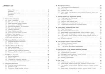
1 Parameter estimationConditionAspirinPlaceboStatisticians do it when it counts.1.1What is Statistics?Statistics is a collection of procedures and principles for gaining and processinginformation in order to make decisions when faced with uncertainty.This course is concerned with “Mathematical Statistics”, i.e., mathematical ideasand tools that are used by statisticians to analyse data. We will study techniques forestimating parameters, fitting models, and testing hypotheses. However, as we studythese techniques we should be aware that a practicing statistician needs more thansimply a knowledge of mathematical techniques. The collection and interpretationof data is a subtle art. It requires common sense. It can sometimes raise philosophical questions. Although this course is primarily concerned with mathematicaltechniques, I will also try, by means of examples and digressions, to introduce youto some of the non-mathematical aspects of Statistics.Statistics is concerned with data analysis: using data to make inferences. It isconcerned with questions like ‘what is this data telling me?’ and ‘what does this datasuggest it is reasonable to believe?’ Two of its principal concerns are parameterestimation and hypothesis testing.Many families of probability distributions depend on a small number of parameters; for example, the Poisson family depends on a single parameter λ and the Normalfamily on two parameters µ and σ. Unless the values of the parameters are knownin advance, they must be estimated from data. One major theme of mathematicalstatistics is the theory of parameter estimation and its use in fitting probabilitydistributions to data. A second major theme of Statistics is hypothesis testing.No heart attack10,93310,845Attacks per 10009.4217.13What can we make of this data? Does it support the hypothesis that aspirinprevents heart attacks?The aspirin study is an example of a controlled experiment. The subjects weredoctors aged 40 to 84 and none knew whether they were taking the aspirin or theplacebo. Statistics is also concerned with analysing data from observational studies.For example, most of us make an intuitive statistical analysis when we use ourprevious experience to help us choose the shortest checkout line at a supermarket.The data analysis of observational studies and experiments is a central componentof decision-making, in science, medicine, business and government.By the way: data is a plural noun referring to a collection of numbers or otherpieces of information to which meaning has been attached.The numbers 1.1, 3.0, 6.5 are not necessarily data. They become so when weare told that they are the muscle weight gains in kg of three athletes who have beentrying a new diet.1.2Example 1.1 Suppose we wish to estimate the proportion p of students in Cambridge who have not showered or bathed for over a day.This poses a number of questions. Who do we mean by students? Suppose timeis limited and we can only interview 20 students in the street. Is it important thatour survey is ‘random’ ? How can we ensure this? Will interviewees be embarrassedto admit if they have not bathed? And even if we can get truthful answers, will webe happy with our estimate if that random sample turns out to include no women,or if it includes only computer scientists?Suppose we find that 5 have not bathed for over a day. We might estimate p byp̂ 5/20 0.25. But how large an error might we expect p̂ to have?Heart attack104189RVs with values in Rn or ZnIn Statistics, our data are modelled by a vector of random variablesX (X1 , X2 , . . . , Xn )where Xi takes values in Z or R.To succeed in this course you should brush up on your knowledge of basic probability: of key distributions and how to make calculations with random variables. Letus review a few facts.When our sample space Ω (a set of possible outcomes) is discrete (finite or countably infinite) we have a random variable (RV) X with values in Z:X : Ω Z.RVs can also take values in R rather than in Z and the sample space Ω can beuncountable.X : Ω R.Example 1.2 A famous study investigated the effects upon heart attacks of takingan aspirin every other day. The results after 5 years wereSince the outcome ω, ω Ω, is random, X is a function whose value, X(ω), isalso random. E.g., to model the experiment of tossing a coin twice we might takeΩ {hh, ht, th, tt}. Then X might be the total number of heads.12

In both cases the distribution function FX of X is defined as:XFX (x) : P(X x) P(ω).{ω : X(ω) x}In the discrete case the probability mass function (pmf) fX of X isfX (k) : P(X k),k Z.SoP(X A) XfX (x),x AA Z.In the continuous case we have the probability density function (pdf) fX of X.In all cases we shall meet, X will have a piecewise smooth pdf such thatZP(X A) fX (x) dx, for nice (measurable) subsets A R.1.3(a) We say that X has the binomial distribution B(n, p), and write X B(n, p),if( n kn kif k {0, . . . , n},k p (1 p)P(X k) 0otherwise.Then E(X) np, var(X) np(1 p). This is the distribution of the number ofsuccesses in n independent trials, each of which has probability of success p.(b) We say that X has the Poisson distribution with parameter λ, and writeX P (λ), if(e λ λk /k! if k {0, 1, 2, . . .},P(X k) 0otherwise.Then E(X) var(X) λ. The Poisson is the limiting distribution of B(n, p) asn and p 0 with λ np.(c) We say that X is standard normal, and write X N (0, 1), ifx AExpectation of X: In the discrete caseXXE(X) : X(ω)P(ω) k P(X k),ω Ωk Zthe first formula being the real definition. In the continuous case the calculationZE(X) X(ω) P(dω)Ωneeds measure theory. However,fX (x) dFX (x)dxSome important random variables1exp( x2 /2),fX (x) ϕ(x) : 2πThenFX (x) ZxfX (y) dy Φ(x) : x .Zxϕ(y) dy. Then E(X) 0, var(X) 1. Φ and ϕ are standard notations.(d) We say that X is normal with mean µ and variance σ 2 , and write X N (µ, σ 2 )if 1(x µ)2fX (x) exp , x .2σ 2σ 2πThen E(X) µ, var(X) σ 2 .except perhaps for finitely many x.(e) We say that X is uniform on [a, b], and write X U [a, b], iffX (x) 1,b ax [a, b].Measure theory shows that for any nice function h on R,ZE h(X) h(x)fX (x) dx .Then E(X) 12 (a b), var(X) Variance of X: If E(X) µ, thenRandom variables X1 , . . . , Xn are called independent if for all x1 , . . . , xn112 (b a)2 .R1.4Independent and IID RVsvar(X) E(X µ)2 E(X 2 ) µ2 .P(X1 x1 ; . . . ; Xn xn ) P(X1 x1 ) · · · P(Xn xn ).34

IID stands for independent identically distributed. Thus if X1 , X2 , . . . , Xnare IID RVs, then they all have the same distribution function and hence the samemean and same variance.We work with the probability mass function (pmf) of X in Zn or probabilitydensity function (pdf) of X in Rn : In most cases, X1 , . . . , Xn are independent, sothat if x (x1 , . . . , xn ) Rn , thenfX (x) fX1 (x1 ) · · · fXn (xn ).1.5Indicating dependence on parametersIf X N (µ, σ 2 ), then we indicate the dependence of the pdf of X on µ and σ 2 bywriting it as 1(x µ)22f (x µ, σ ) exp 2σ 2(2πσ 2 )1/2Or if X (X1 , . . . , Xn ), where X1 , . . . , Xn are IID N (µ, σ 2 ), then we would havef (x µ, σ 2 ) 1kx µ1k2exp 2σ 2(2πσ 2 )n/21.7Unbiased estimatorsAn estimator of a parameter θ is a function T T (X) which we use to estimate θfrom an observation of X. T is said to be unbiased ifE(T ) θ.The expectation above is taken over X. Once the actual data x is observed, t T (x)is the estimate of θ obtained via the estimator T .Example 1.3 Suppose X1 , . . . , Xn arePIID B(1, p) and p is unknown. Consider theestimator for p given by p̂(X) X̄ i Xi /n. Then p̂ is unbiased, since 111Ep̂(X) E(X1 · · · Xn ) (EX1 · · · EXn ) np p .nnnAnother possible unbiased estimator for p is p̃ 13 (X1 2X2 ) (i.e., we ignoremost of the data.) It is also unbiased since 111Ep̃(X) E (X1 2X2 ) (EX1 2EX2 ) (p 2p) p .333Intuitively, the first estimator seems preferable.where µ1 denotes the vector (µ, µ, . . . , µ) .In general, we write f (x θ) to indicate that the pdf depends on a parameter θ.θ may be a vector of parameters. In the above θ (µ, σ 2 ) . An alternative notationwe will sometimes employ is fθ (x).The set of distributions with densities fθ (x), θ Θ, is called a parametricfamily. E.g.,, there is a parametric family of normal distributions, parameterisedby values of µ, σ 2 . Similarly, there is a parametric family of Poisson distributions,parameterised by values of λ.1.8Sums of independent RVsIn the above calculations we have used the fact the expectation of a sum of randomvariables is the sum of their expectations. It is always true (even when X1 , . . . , Xnare not independent) thatE(X1 · · · Xn ) E(X1 ) · · · E(Xn ),and for linear combinations of RVs1.6The notion of a statisticE(a1 X1 · · · an Xn ) a1 E(X1 ) · · · an E(Xn ).A statistic, T (x), is any function of the data. E.g., given the data x (x1 , . . . , xn ),four possible statistics are1(x1 · · · xn ),nmax xi ,ix1 x3log x4 ,xn2004 10 min xi .iClearly, some statistics are more natural and useful than others. The first of thesewould be useful for estimating µ if the data are samples from a N (µ, 1) distribution.The second would be useful for estimating θ if the data are samples from U [0, θ].5If X1 , X2 , . . . , Xn are independent, thenE(X1 X2 . . . Xn ) E(X1 )E(X2 ) · · · E(Xn ),var(X1 · · · Xn ) var(X1 ) · · · var(Xn ),and for linear combinations of independent RVsvar(a1 X1 · · · an Xn ) a21 var(X1 ) · · · a2n var(Xn ).6

1.9More important random variables(a) We say that X is geometric with parameter p, if(p(1 p)k 1 if k {1, 2, . . .},P(X k) 0otherwise.Then E(X) 1/p and var(X) (1 p)/p2 . X is the number of the toss on whichwe first observe a head if we toss a coin which shows heads with probability p.(b) We say that X is exponential with rate λ, and write X E(λ), if(λe λx if x 0,fX (x) 0otherwise.Then E(X) λ 1 , var(X) λ 2 .The geometric and exponential distributions are discrete and continuous analogues. They are the unique ‘memoryless’ distributions, in the sense that P(X t s X t) P(X s). The exponential is the distribution of the time betweensuccessive events of a Poisson process.(c) We say that X is gamma(n, λ) if(λn xn 1 e λx /(n 1)! if x 0,fX (x) 0otherwise.X has the distribution of the sum of n IID RVs that have distribution E(λ). SoE(λ) gamma(1, λ). E(X) nλ 1 and var(X) nλ 2 .This also makesR sense for real n 0 (and λ 0), if we interpret (n 1)! as Γ(n),where Γ(n) 0 xn 1 e x dx.(d) We say that X is beta(a, b) if(fX (x) 1B(a,b)0xa 1 (1 x)b 1if 0 x 1,otherwise.Here B(a, b) Γ(a)Γ(b)/Γ(a b). ThenE(X) 1.10a,a bvar(X) ab.(a b 1)(a b)2The weak law of large numbers is that for ǫ 0,P( Sn /n µ ǫ) 0, as n .The strong law of large numbers is thatP(Sn /n µ) 1 .1.11The Central Limit TheoremSuppose X1 , X2 , . . . are as above. Define the standardized version Sn of Sn asSn Sn nµ ,σ nso that E(Sn ) 0, var(Sn ) 1.Then for large n, Sn is approximately standard normal: for a b, lim P(a Sn b) Φ(b) Φ(a) lim P nµ aσ n Sn nµ bσ n .n n In particular, for large n, P( Sn nµ 1.96σ n) 95%since Φ(1.96) 0.975 and Φ( 1.96) 0.025.1.12Poisson process of rate λThe Poisson process is used to model a process of arrivals: of people to a supermarketcheckout, calls at telephone exchange, etc.Arrivals happen at timesT1 , T1 T2 , T1 T2 T3 , . . .where T1 , T2 , . . . are independent and each exponentially distributed with parameterλ. Numbers of arrivals in disjoint intervals are independent RVs, and the number ofarrivals in any interval of length t has the P (λt) distribution. The timeSn T 1 T 2 · · · T n2of the nth arrival has the gamma(n, λ) distribution, and 2λSn X2n.Laws of large numbersSuppose X1 , X2 , . . . is a sequence of IID RVs, each having finite mean µ and varianceσ 2 . LetSn : X1 X2 · · · Xn , so that E(Sn ) nµ, var(Sn ) nσ 2 .78

2 Maximum likelihood estimationWhen it is not in our power to follow what is true, we oughtto follow what is most probable. (Descartes)2.1Maximum likelihood estimationSuppose that the random variable X has probability density function f (x θ). Giventhe observed value x of X, the likelihood of θ is defined bylik(θ) f (x θ) .nYi 1(b) X B(n, p), n known, p to be estimated.Here n xp (1 p)n x · · · x log p (n x) log(1 p) .log p(x n, p) logxThis is maximized whereThus we are considering the density as a function of θ, for a fixed x. In the caseof multiple observations, i.e., when x (x1 , . . . , xn ) is a vector of observed valuesof X1 , . . . , Xn , we assume, unless otherwise stated, that X1 , . . . , Xn are IID; in thiscase f (x1 , . . . , xn θ) is the product of the marginals,lik(θ) f (x1 , . . . , xn θ) which equals 2/27, 3/32, 12/125, 5/54 for k 3, 4, 5, 6, and decreases thereafter.Hence the maximum likelihood estimate is k̂ 5. Note that although we have seenonly 3 colours the maximum likelihood estimate is that there are 2 colours we havenot yet seen.f (xi θ) .It makes intuitive sense to estimate θ by whatever value gives the greatest likelihood to the observed data. Thus the maximum likelihood estimate θ̂(x) of θis defined as the value of θ that maximizes the likelihood. Then θ̂(X) is called themaximum likelihood estimator (MLE) of θ.Of course, the maximum likelihood estimator need not exist, but in many examples it does. In practice, we usually find the MLE by maximizing log f (x θ), whichis known as the loglikelihood.x n x 0,p̂1 p̂so the MLE of p is p̂ X/n. Since E[X/n] p the MLE is unbiased.(c) X B(n, p), p known, n to be estimated.Now we want to maximize n xp(x n, p) p (1 p)n xxwith respect to n, n {x, x 1, . . .}. To do this we look at the ratio n 1 xp (1 p)n 1 xp(x n 1, p)(1 p)(n 1) xn x .n xp(x n, p)n 1 xp(1 p)xThis is monotone decreasing in n. Thus p(x n, p) is maximized by the least n forwhich the above expression is 1, i.e., the least n such that(1 p)(n 1) n 1 x n 1 x/p ,giving a MLE of n̂ [X/p]. Note that if x/p happens to be an integer then bothn x/p 1 and n x/p maximize p(x n, p). Thus the MLE need not be unique.Examples 2.1(a) Smarties are sweets that come in k equally frequent colours. Suppose we donot know k. We sequentially examine 3 Smarties and they are red, green, red. Thelikelihood of this data, x the second Smartie differs in colour from the first but thethird Smartie matches the colour of the first, is k 1 1lik(k) p(x k) P(2nd differs from 1st)P(3rd matches 1st) kk(d) X1 , . . . , Xn geometric(p), p to be estimated.Because the Xi are IID their joint density is the product of the marginals, so!nnYXxi 1log f (x1 , . . . , xn p) log (1 p)p xi n log(1 p) n log p .i 1with a maximum where 2 (k 1)/k ,which equals 1/4, 2/9, 3/16 for k 2, 3, 4, and continues to decrease for greater k.Hence the maximum likelihood estimate is k̂ 2.Suppose a fourth Smartie is drawn and it is orange. Nowlik(k) (k 1)(k 2)/k 3 ,9i 1Pxi n n 0.1 p̂p̂iSo the MLE is p̂ X̄ 1 . This MLE is biased. For example, in the case n 1,E[1/X1 ] X1p(1 p)x 1 p log p p .x1 px 1Note that E[1/X1 ] does not equal 1/EX1 .10

2.2Sufficient statisticsThe MLE, if it exists, is always a function of a sufficient statistic. The informal notion of a sufficient statistic T T (X1 , . . . , Xn ) is that it summarises all informationin {X1 , . . . , Xn } which is relevant to inference about θ.Formally, the statistic T T (X) is said to be sufficient for θ Θ if, for eacht, Pθ X · T (X) t does not depend on θ. I.e., the conditional distribution ofX1 , . . . , Xn given T (X) t does not involve θ. Thus to know more about x thanthat T (x) t is of no additional help in making any inference about θ.Theorem 2.2 The statistic T is sufficient for θ if and only if f (x θ) can be expressed as f (x θ) g T (x), θ h(x).This is called the factorization criterion.Proof. We give a proof for the case that the sample space is discrete. A continuous sample space needs measure theory. Suppose f (x θ) Pθ (X x) has thefactorization above and T (x) t. Then g T (x), θ h(x)Pθ (X x) P Pθ X x T (X) t Pθ T (X) tx:T (x) t g T (x), θ h(x) Ph(x)g(t, θ)h(x) Pg(t,θ)h(x)x:T (x) tx:T (x) t h(x)which does not depend on θ. Conversely, if T is sufficient and T (x) t, Pθ (X x) Pθ T (X) t Pθ X x T (X) twhere by sufficiency the second factor does not depend on θ. So we identify the firstand second terms on the r.h.s. as g(t, θ) and h(x) respectively.The MLE is found by maximizing f (x λ), and soPxidlog f (x λ) i n 0.dλλ̂λ λ̂Hence λ̂ X̄. It is easy to check that λ̂ is unbiased.Note that the MLE is always a functi

The aim of this course is to aquaint you with the basics of mathematical statistics: the ideas of estimation, hypothesis testing and statistical modelling. . Probability and Statistics, 3rd edition, Addison-Wesley, 2001, ISBN . 6th Edition, 2002, ISBN -534-37741-6. J. A. Rice, Mathematical Statistics and Data Analysis, 2nd edition, Duxbury .