Transcription
Creating R Packages: A TutorialFriedrich LeischDepartment of Statistics, Ludwig-Maximilians-Universität München, andR Development Core Team, Friedrich.Leisch@R-project.orgSeptember 14, 2009This is a reprint of an article that has appeared in: Paula Brito, editor, Compstat 2008-Proceedingsin Computational Statistics. Physica Verlag, Heidelberg, Germany, 2008.AbstractThis tutorial gives a practical introduction to creating R packages. We discuss how objectoriented programming and S formulas can be used to give R code the usual look and feel,how to start a package from a collection of R functions, and how to test the code once thepackage has been created. As running example we use functions for standard linear regressionanalysis which are developed from scratch.Keywords:1R packages, statistical computing, software, open sourceIntroductionThe R packaging system has been one of the key factors of the overall success of the R project (RDevelopment Core Team 2008). Packages allow for easy, transparent and cross-platform extensionof the R base system. An R package can be thought of as the software equivalent of a scientificarticle: Articles are the de facto standard to communicate scientific results, and readers expectthem to be in a certain format. In Statistics, there will typically be an introduction including aliterature review, a section with the main results, and finally some application or simulations.But articles need not necessarily be the usual 10–40 pages communicating a novel scientific ideato the peer group, they may also serve other purposes. They may be a tutorial on a certain topic(like this paper), a survey, a review etc. The overall format is always the same: text, formulasand figures on pages in a journal or book, or a PDF file on a web server. Contents and quality willvary immensely, as will the target audience. Some articles are intended for a world-wide audience,some only internally for a working group or institution, and some may only be for private use ofa single person.R packages are (after a short learning phase) a comfortable way to maintain collections of Rfunctions and data sets. As an article distributes scientific ideas to others, a package distributesstatistical methodology to others. Most users first see the packages of functions distributed withR or from CRAN. The package system allows many more people to contribute to R while stillenforcing some standards. But packages are also a convenient way to maintain private functionsand share them with your colleagues. I have a private package of utility function, my working grouphas several “experimental” packages where we try out new things. This provides a transparentway of sharing code with co-workers, and the final transition from “playground” to productioncode is much easier.But packages are not only an easy way of sharing computational methods among peers, theyalso offer many advantages from a system administration point of view. Packages can be dynamically loaded and unloaded on runtime and hence only occupy memory when actually used.Installations and updates are fully automated and can be executed from inside or outside R. And1
last but not least the packaging system has tools for software validation which check that documentation exists and is technically in sync with the code, spot common errors, and check thatexamples actually run.Before we start creating R packages we have to clarify some terms which sometimes get confused:Package: An extension of the R base system with code, data and documentation in standardizedformat.Library: A directory containing installed packages.Repository: A website providing packages for installation.Source: The original version of a package with human-readable text and code.Binary: A compiled version of a package with computer-readable text and code, may work onlyon a specific platform.Base packages: Part of the R source tree, maintained by R Core.Recommended packages: Part of every R installation, but not necessarily maintained by RCore.Contributed packages: All the rest. This does not mean that these packages are necessarily oflesser quality than the above, e.g., many contributed packages on CRAN are written andmaintained by R Core members. We simply try to keep the base distribution as lean aspossible.See R Development Core Team (2008a) for the full manual on R installation issues, and Ligges(2003) for a short introduction.The remainder of this tutorial is organized as follows: As example we implement a function forlinear regression models. We first define classes and methods for the statistical model, includinga formula interface for model specification. We then structure the pieces into the form of anR package, show how to document the code properly and finally discuss the tools for packagevalidation and distribution. This tutorial is meant as a starting point on how to create an Rpackage, see R Development Core Team (2008b) for the full reference manual. Note that Rimplements a dialect of the S programming language (Becker et al 1988), in the following we willprimarily use the name “S” when we speak of the language, and “R” when the complete R softwareenvironment is meant or extensions of the S language which can only be found in R.2R code for linear regressionAs running example in this tutorial we will develop R code for the standard linear regression modely x0 β , N (0, σ 2 )Our goal is not to implement all the bells and whistles of the standard R function lm() for theproblem, but to write a simple function which computes the OLS estimate and has a “professionallook and feel” in the sense that the interface is similar to the interface of lm().If we are given a design matrix X and response vector y then the OLS estimate is of courseβ̂ (X 0 X) 1 X 0 ywith covariance matrixvar(β̂) σ 2 (X 0 X) 1For numerical reasons it is not advisable to compute β̂ using the above formula, it is betterto use, e.g., a QR decomposition or any other numerically good way to solve a linear system ofequations (e.g., Gentle 1998). Hence, a minimal R function for linear regression is2
linmodEst - function(x, y){## compute QR-decomposition of xqx - qr(x)## compute (x’x) (-1) x’ycoef - solve.qr(qx, y)## degrees of freedom and standard deviation of residualsdf - nrow(x)-ncol(x)sigma2 - sum((y - x%*%coef) 2)/df## compute sigma 2 * (x’x) -1vcov - sigma2 * chol2inv(qx qr)colnames(vcov) - rownames(vcov) - colnames(x)list(coefficients coef,vcov vcov,sigma sqrt(sigma2),df df)}If we use this function to predict heart weight from body weight in the classic Fisher cats datafrom package MASS (Venables & Ripley 2002), we getR data(cats, package "MASS")R linmodEst(cbind(1, cats Bwt), cats Hwt) coefficients[1] -0.3566624 4.0340627 vcov[,1][,2][1,] 0.4792475 -0.17058197[2,] -0.1705820 0.06263081 sigma[1] 1.452373 df[1] 142The standard R function for linear models:R lm1 - lm(Hwt Bwt, data cats)R lm1Call:lm(formula Hwt Bwt, data cats)Coefficients:(Intercept)Bwt-0.35674.0341R vcov(lm1)(Intercept)Bwt(Intercept)0.4792475 -0.17058197Bwt-0.1705820 0.062630813
The numerical estimates are exactly the same, but our code lacks a convenient user interface:1. Prettier formatting of results.2. Add utilities for fitted model like a summary() function to test for significance of parameters.3. Handle categorical predictors.4. Use formulas for model specification.Object oriented programming helps us with issues 1 and 2, formulas with 3 and 4.3Object oriented programming in R3.1S3 and S4Our function linmodEst returns a list with four named elements, the parameter estimates andtheir covariance matrix, and the standard deviation and degrees of freedom of the residuals. Fromthe context it is clear to us that this is a linear model fit, however, nobody told the computer sofar. For the computer this is simply a list containing a vector, a matrix and two scalar values.Many programming languages, including S, use so-called1. classes to define how objects of a certain type look like, and2. methods to define special functions operating on objects of a certain classA class defines how an object is represented in the program, while an object is an instance of theclass that exists at run time. In our case we will shortly define a class for linear model fits. Theclass is the abstract definition, while every time we actually use it to store the results for a givendata set, we create an object of the class.Once the classes are defined we probably want to perform some computations on objects. Inmost cases we do not care how the object is stored internally, the computer should decide how toperform the tasks. The S way of reaching this goal is to use generic functions and method dispatch:the same function performs different computations depending on the classes of its arguments.S is rare because it is both interactive and has a system for object-orientation. Designingclasses clearly is programming, yet to make S useful as an interactive data analysis environment,it makes sense that it is a functional language. In “real” object-oriented programming (OOP)languages like C or Java class and method definitions are tightly bound together, methodsare part of classes (and hence objects). We want incremental and interactive additions like userdefined methods for pre-defined classes. These additions can be made at any point in time, evenon the fly at the command line prompt while we analyze a data set. S tries to make a compromisebetween object orientation and interactive use, and although compromises are never optimal withrespect to all goals they try to reach, they often work surprisingly well in practice.The S language has two object systems, known informally as S3 and S4.S3 objects, classes and methods have been available in R from the beginning, they are informal,yet “very interactive”. S3 was first described in the “White Book” (Chambers & Hastie1992).S4 objects, classes and methods are much more formal and rigorous, hence “less interactive”. S4was first described in the “Green Book” (Chambers 1998). In R it is available through themethods package, attached by default since version 1.7.0.S4 provides formal object oriented programming within an interactive environment. It can helpa lot to write clean and consistent code, checks automatically if objects conform to class definitions,and has much more features than S3, which in turn is more a set of naming conventions than atrue OOP system, but it is sufficient for most purposes (take almost all of R as proof). BecauseS3 is much easier to learn than S4 and sufficient for our purposes, we will use it throughout thistutorial.4
3.2The S3 systemIf we look at the following R session we already see the S3 system of classes and methods at work:R x - rep(0:1, c(10, 20))R x[1] 0 0 0 0 0 0 0 0 0 0 1 1 1 1 1 1 1 1 1 1 1 .R class(x)[1] "integer"R summary(x)Min. 1st Qu. MedianMean 3rd Qu.Max.0.0000 0.0000 1.0000 0.6667 1.0000 1.0000R y - as.factor(x)R class(y)[1] "factor"R summary(y)0 110 20Function summary() is a generic function which performs different operations on objects of differentclasses. In S3 only the class of the first argument to a generic function counts. For objects ofclass "integer" (or more generally "numeric") like x the five number summary plus the mean iscalculated, for objects of class "factor" like y a table of counts.Classes are attached to objects as an attribute:R attributes(y) levels[1] "0" "1" class[1] "factor"In S3 there is no formal definition of a class. To create an object from a new class, one simplysets the class attribute of an object to the name of the desired class:R myx - xR class(myx) - "myvector"R class(myx)[1] "myvector"Of course in most cases it is useless to define a class without defining any methods for theclass, i.e., functions which do special things for objects from the class. In the simplest case onedefines new methods for already existing generic functions like print(), summary() or plot().These are available for objects of many different classes and should do the following:print(x, .): this method is called, when the name of an object is typed at the prompt. Fordata objects it usually shows the complete data, for fitted models a short description of themodel (only a few lines).summary(x, .): for data objects summary statistics, for fitted models statistics on parameters,residuals and model fit (approx. one screen). The summary method should not directly createscreen output, but return an object which is then print()ed.plot(x, y, .): create a plot of the object in a graphics device.Generic functions in S3 take a look at the class of their first argument and do method dispatchbased on a naming convention: foo() methods for objects of class "bar" are called foo.bar(),5
e.g., summary.factor() or print.myvector(). If no bar method is found, S3 searches forfoo.default(). Inheritance can be emulated by using a class vector.Let us return to our new class called "myvector". To define a new print() method for ourclass, all we have to do is define a function called print.myvector():print.myvector - function(x, .){cat("This is my vector:\n")cat(paste(x[1:5]), ".\n")}If we now have a look at x and myx they are printed differently:R x[1] 0 0 0 0 0 0 0 0 0 0 1 1 1 1 1 1 1 1 1 1 1 1 1 1 1 1 1 1 1 1R myxThis is my vector:0 0 0 0 0 0 0 0 0 0 .So we see that S3 is highly interactive, one can create new classes and change methods definitions on the fly, and it is easy to learn. Because everything is just solved by naming conventions(which are not checked by R at runtime1 ), it is easy to break the rules. A simple example: Function lm() returns objects of class "lm". Methods for that class of course expect a certain formatfor the objects, e.g., that they contain regression coefficients etc as the following simple exampleshows:R nolm - "This is not a linear model!"R class(nolm) - "lm"R nolmCall:NULLNo coefficientsWarning messages:1: In x call : operator is invalid foratomic vectors, returning NULL2: In object coefficients : operator is invalid for atomic vectors,returning NULLThe computer should detect the real problem: a character string is not an "lm" object. S4 providesfacilities for solving this problem, however at the expense of a steeper learning curve.In addition to the simple naming convention on how to find objects, there are several moreconventions which make it easier to use methods in practice: A method must have all the arguments of the generic, including . if the generic does. A method must have arguments in exactly the same order as the generic. If the generic specifies defaults, all methods should use the same defaults.The reason for the above rules is that they make it less necessary to read the documentation forall methods corresponding to the same generic. The user can rely on common rules, all methodsoperate “as similar” as possible. Unfortunately there are no rules without exceptions, as we willsee in one of the next sections . . .1 Thereis checking done as part of package quality control, see the section on R CMD check later in this tutorial.6
3.3Classes and methods for linear regressionWe will now define classes and methods for our linear regression example. Because we want towrite a formula interface we make our main function linmod() generic, and write a default methodwhere the first argument is a design matrix (or something which can be converted to a matrix).Later-on we will add a second method where the first argument is a formula.A generic function is a standard R function with a special body, usually containing only a callto UseMethod:linmod - function(x, .) UseMethod("linmod")To add a default method, we define a function called linmod.default():linmod.default - function(x, y, .){x - as.matrix(x)y - as.numeric(y)est - linmodEst(x, y)est fitted.values - as.vector(x %*% est coefficients)est residuals - y - est fitted.valuesest call - match.call()class(est) - "linmod"est}This function tries to convert its first argument x to a matrix, as.matrix() will throw an error ifthe conversion is not successful2 , similarly for the conversion of y to a numeric vector. We thencall our function for parameter estimation, and add fitted values, residuals and the function callto the results. Finally we set the class of the return object to "linmod".Defining the print() method for our class asprint.linmod - function(x, .){cat("Call:\n")print(x call)cat("\nCoefficients:\n")print(x coefficients)}makes it almost look like the real thing:R x cbind(Const 1, Bwt cats Bwt)R y cats HwR mod1 - linmod(x, y)R mod1Call:linmod.default(x x, y y)Coefficients:ConstBwt-0.3566624 4.03406272 Whatwe do not catch here is conversion to a non-numeric matrix like character strings.7
Note that we have used the standard names "coefficients", "fitted.values" and"residuals" for the elements of our class "linmod". As a bonus on the side we get methodsfor several standard generic functions for free, because their default methods work for our class:R coef(mod1)ConstBwt-0.3566624 4.0340627R fitted(mod1)[1] 7.711463 7.711463 7.711463 8.114869 8.114869 8.114869 .R resid(mod1)[1] -0.7114630 -0.3114630 1.7885370 -0.9148692 -0.8148692 .The notion of functions returning an object of a certain class is used extensively by the modelling functions of S. In many statistical packages you have to specify a lot of options controllingwhat type of output you want/need. In S you first fit the model and then have a set of methodsto investigate the results (summary tables, plots, . . . ). The parameter estimates of a statisticalmodel are typically summarized using a matrix with 4 columns: estimate, standard deviation, z(or t or . . . ) score and p-value. The summary method computes this matrix:summary.linmod - function(object, .){se - sqrt(diag(object vcov))tval - coef(object) / seTAB - cbind(Estimate coef(object),StdErr se,t.value tval,p.value 2*pt(-abs(tval), df object df))res - list(call object call,coefficients TAB)class(res) - "summary.linmod"res}The utility function printCoefmat() can be used to print the matrix with appropriate roundingand some decoration:print.summary.linmod - function(x, .){cat("Call:\n")print(x call)cat("\n")printCoefmat(x coefficients, P.value TRUE, has.Pvalue TRUE)}The results isR summary(mod1)Call:linmod.default(x x, y y)EstimateConst -0.35666StdErr t.value p.value0.69228 -0.5152 0.60728
Bwt4.03406--Signif. codes:0.25026 16.1194 2e-16 ***0 *** 0.001 ** 0.01 * 0.05 . 0.11Separating computation and screen output has the advantage, that we can use all values if neededfor later computations. E.g., to obtain the p-values we can useR coef(summary(mod1))[,4]ConstBwt6.072131e-01 6.969045e-344S FormulasThe unifying interface for selecting variables from a data frame for a plot, test or model are Sformulas. The most common formula is of typey x1 x2 x3The central object that is usually created first from a formula is themodel.frame, a data frame containing only the variables appearing in the formula, together withan interpretation of the formula in theterms attribute. It tells us whether there is a response variable (always the first column of themodel.frame), an intercept, . . .The model.frame is then used to build the design matrix for the model and get the response.Our code shows the simplest handling of formulas, which however is already sufficient for manyapplications (and much better than no formula interface at all):linmod.formula - function(formula, data list(), .){mf - model.frame(formula formula, data data)x - model.matrix(attr(mf, "terms"), data mf)y - model.response(mf)est - linmod.default(x, y, .)est call - match.call()est formula - formulaest}The above function is an example for the most common exception to the rule that all methodsshould have the same arguments as the generic and in the same order. By convention formulamethods have arguments formula and data (rather than x and y), hence there is at least adifference in names of the first argument: x in the generic, formula in the formula method. Thisexception is hard-coded in the quality control tools of R CMD check described below.The few lines of R code above give our model access to the wide variety of design matrices Sformulas allow us to specify. E.g., to fit a model with main effects and an interaction term forbody weight and sex we can useR summary(linmod(Hwt Bwt*Sex, data cats))Call:linmod.formula(formula Hwt Bwt * Sex, data cats)(Intercept)Estimate2.98131StdErr t.valuep.value1.84284 1.6178 0.10796059
Bwt2.63641SexM-4.16540Bwt:SexM1.67626--Signif. codes: 0 ***0.77590 3.3979 0.0008846 ***2.06176 -2.0203 0.0452578 *0.83733 2.0019 0.0472246 *0.001 ** 0.01 * 0.05 . 0.11The last missing methods most statistical models in S have are a plot() and predict()method. For the latter a simple solution could bepredict.linmod - function(object, newdata NULL, .){if(is.null(newdata))y - fitted(object)else{if(!is.null(object formula)){## model has been fitted using formula interfacex - model.matrix(object formula, newdata)}else{x - newdata}y - as.vector(x %*% coef(object))}y}which works for models fitted with either the default method (in which case newdata is assumedto be a matrix with the same columns as the original x matrix), or for models fitted using theformula method (in which case newdata will be a data frame). Note that model.matrix() canalso be used directly on a formula and a data frame rather than first creating a model.frame.The formula handling in our small example is rather minimalistic, production code usuallyhandles much more cases. We did not bother to think about treatment of missing values, weights,offsets, subsetting etc. To get an idea of more elaborate code for handling formulas, one can lookat the beginning of function lm() in R.5R packagesNow that we have code that does useful things and has a nice user interface, we may want to shareour code with other people, or simply make it easier to use ourselves. There are two popular waysof starting a new package:1. Load all functions and data sets you want in the package into a clean R session, and runpackage.skeleton(). The objects are sorted into data and functions, skeleton help filesare created for them using prompt() and a DESCRIPTION file is created. The function thenprints out a list of things for you to do next.2. Create it manually, which is usually faster for experienced developers.5.1Structure of a packageThe extracted sources of an R package are simply a directory3 somewhere on your hard drive. Thedirectory has the same name as the package and the following contents (all of which are describedin more detail below):3 Directoriesare sometimes also called folders, especially on Windows.10
A file named DESCRIPTION with descriptions of the package, author, and license conditionsin a structured text format that is readable by computers and by people. A man/ subdirectory of documentation files. An R/ subdirectory of R code. A data/ subdirectory of datasets.Less commonly it contains A src/ subdirectory of C, Fortran or C source. tests/ for validation tests. exec/ for other executables (eg Perl or Java). inst/ for miscellaneous other stuff. The contents of this directory are completely copied tothe installed version of a package. A configure script to check for other required software or handle differences between systems.All but the DESCRIPTION file are optional, though any useful package will have man/ and at leastone of R/ and data/. Note that capitalization of the names of files and directories is important,R is case-sensitive as are most operating systems (except Windows).5.2Starting a package for linear regressionTo start a package for our R code all we have to do is run function package.skeleton() andpass it the name of the package we want to create plus a list of all source code files. If no sourcefiles are given, the function will use all objects available in the user workspace. Assuming that allfunctions defined above are collected in a file called linmod.R, the corresponding call isR package.skeleton(name "linmod", code files "linmod.R")Creating directories .Creating DESCRIPTION .Creating Read-and-delete-me .Copying code files .Making help files .Done.Further steps are described in ’./linmod/Read-and-delete-me’.which already tells us what to do next. It created a directory called "linmod" in the currentworking directory, a listing can be seen in Figure 1. R also created subdirectories man and R,copied the R code into subdirectory R and created stumps for help file for all functions in thecode.File Read-and-delete-me contains further instructions:* Edit the help file skeletons in ’man’, possiblycombining help files for multiple functions.* Put any C/C /Fortran code in ’src’.* If you have compiled code, add a .First.lib() functionin ’R’ to load the shared library.* Run R CMD build to build the package tarball.* Run R CMD check to check the package tarball.Read "Writing R Extensions" for more information.We do not have any C or Fortran code, so we can forget about items 2 and 3. The code is alreadyin place, so all we need to do is edit the DESCRIPTION file and write some help pages.11
Figure 1: Directory listing of package linmod after running function package.skeleton().12
5.3The package DESCRIPTION fileAn appropriate DESCRIPTION for our package isPackage: linmodTitle: Linear RegressionVersion: 1.0Date: 2008-05-13Author: Friedrich LeischMaintainer: Friedrich Leisch Friedrich.Leisch@R-project.org Description: This is a demo package for the tutorial "Creating RPackages" to Compstat 2008 in Porto.Suggests: MASSLicense: GPL-2The file is in so called Debian-control-file format, which was invented by the Debian Linux distribution (http://www.debian.org) to describe their package. Entries are of formKeyword: Valuewith the keyword always starting in the first column, continuation lines start with one ore morespace characters. The Package, Version, License, Description, Title, Author, and Maintainerfields are mandatory, the remaining fields (Date, Suggests, .) are optional.The Package and Version fields give the name and the version of the package, respectively.The name should consist of letters, numbers, and the dot character and start with a letter. Theversion is a sequence of at least two (and usually three) non-negative integers separated by singledots or dashes.The Title should be no more than 65 characters, because it will be used in various packagelistings with one line per package. The Author field can contain any number of authors in free textformat, the Maintainer field should contain only one name plus a valid email address (similarto the “corresponding author” of a paper). The Description field can be of arbitrary length.The Suggests field in our example means that some code in our package uses functionality frompackage MASS, in our case we will use the cats data in the example section of help pages. Astronger form of dependency can be specified in the optional Depends field listing packages whichare necessary to run our code.The License can be free text, if you submit the package to CRAN or Bioconductor anduse a standard license, we strongly prefer that you use a standardized abbreviation like GPL-2which stands for “GNU General Public License Version 2”. A list of license abbreviations Runderstands is given in the manual “Writing R Extensions” (R Development Core Team 2008b).The manual also contains the full documentation for all possible fields in package DESCRIPTIONfiles. The above is only a minimal example, much more meta-information about a package as wellas technical details for package installation can be stated.5.4R documentation filesThe sources of R help files are in R documentation format and have extension .Rd. The format issimilar to LATEX, however processed by R and hence not all LATEX commands are available, in factthere is only a very small subset. The documentation files can be converted into HTML, plaintext, GNU info format, and LATEX. They can also be converted into the old nroff-based S helpformat.A joint help page for all our functions is shown in Figure 2. First the name of the help page,then aliases for all topics the page documents. The title should again be only one line because itis used for the window title in HTML browsers. The descriptions should be only 1–2 paragraphs,if more text is needed it should go into the optional details section not shown in the example.Regular R users will immediately recognize most sections of Rd files from reading other help pages.The usage section should be plain R code with additional markup for methods:13
mmary.linmod}\title{Linear Regression}\description{Fit a linear regression model.}\usage{linmod(x, .)\method{linmod}{default}(x, y, .)\method{linmod}{formula}(formula, data list(), .)\method{print}{linmod}(x, .)\method{summary}{linmod}(object, .)\method{predict}{linmod}(object, newdata NULL, .)}\arguments{\item{x}{ a numeric design matrix for the model. }\item{y}{ a numeric vector of responses. }\item{formula}{ a symbolic description of the model to be fit. }\item{data}{ an optional data frame containing the variables in the model. }\item{object}{ an object of class \code{"linmod"}, i.e., a fitted model. }\item{\dots}{ not used. }}\value{An object of class \code{logreg}, basically a list including elements\item{coefficients}{ a named vector of coefficients }\item{vcov}{ covariance matrix of coefficients }\item{fitted.values}{ fitted values }\item{residuals}{ residuals }}\author{Friedrich Leisch}\examples{data(cats, package "MASS")mod1 - linmod(Hwt Bwt*Sex, data cats)mod1summary(mod1)}\keyword{regression}Figure 2: Help page
Jun 24, 2022