Transcription
Web-Scale Computer Vision using MapReduce forMultimedia Data MiningBrandyn White, Tom Yeh, Jimmy Lin, and Larry DavisUniversity of MarylandCollege Park, MD 20742bwhite@cs.umd.eduABSTRACTThis work explores computer vision applications of the MapReduce framework that are relevant to the data mining community. An overview of MapReduce and common designpatterns are provided for those with limited MapReducebackground. We discuss both the high level theory and thelow level implementation for several computer vision algorithms: classifier training, sliding windows, clustering, bagof-features, background subtraction, and image registration.Experimental results for the k-means clustering and singleGaussian background subtraction algorithms are performedon a 410 node Hadoop cluster.Categories and Subject DescriptorsI.4.0 [Image Processing and Computer Vision]: General; D.1.3 [Programming Techniques]: Concurrent ProgrammingGeneral TermsAlgorithms, Performance, Experimentation.KeywordsMapReduce, computer vision, background subtraction, image registration, clustering, bag-of-features, cloud computing.1.INTRODUCTIONThe amount of available image and video data is increasing dramatically due to the prevalence of social networks,surveillance cameras, and satellite imagery. The currentchallenge is how to effectively manage the computation andstorage requirements imposed by the influx of data. Thetrend towards many-core processors and multi-processor systems is thwarted by the complexity in developing applications that effectively utilize them. A classic solution is todevelop a distributed application using the message passing interface (MPI), which provides fine-grained control overPermission to make digital or hard copies of all or part of this work forpersonal or classroom use is granted without fee provided that copies arenot made or distributed for profit or commercial advantage and that copiesbear this notice and the full citation on the first page. To copy otherwise, torepublish, to post on servers or to redistribute to lists, requires prior specificpermission and/or a fee.MDMKDD’10, July 25, 2010, Washington, DC, USACopyright 2010 ACM 978-1-4503-0220-3 . 10.00.the execution of parallel applications. However, this levelof abstraction adds verbosity and complexity that can exceed that of the desired computation. The MapReduce [5]framework provides a higher level of abstraction than MPIwhile being applicable to many data-intensive batch processing problems. MapReduce provides a simple programmingmodel, a distributed file system [8], job management, andcluster management.Developing and maintaining a computer cluster is a costlyundertaking with a multitude of considerations: power, cooling, support, physical space, hardware, and software. The“utility computing” [18] model replaces these complexitieswith a fixed cost for the resources used, reducing the barrier to entry for researchers and small companies. Moreover,vendor support is available for virtualized MapReduce clusters, further increasing their accessibility.The use of large datasets to ‘let the data do the work’has been gaining popularity. In the field of computationallinguistics, Banko and Brill [1] showed that the most effective algorithms for natural language disambiguation for largedatasets need not be the most effective for small datasets.Brants et al. [2] proposed the “Stupid Backoff” smoothingmethod that approaches the quality of Kneser-Ney givena large input set and was evaluated on 2 trillion tokens.Torallba et al. [20] reported similar findings that by increasing the number of available images, simple nearest neighboralgorithms can produce results comparable to the traditionalViola & Jones method on the person detection task.In this paper, we explore various MapReduce algorithmsfor computer vision tasks. To our knowledge, this is the firstexplication of MapReduce algorithms in this domain. Thiswork is organized as follows. Section 3 gives an overviewof the MapReduce framework and common design patternsare provided for those with limited MapReduce background.Issues related to posing computer vision algorithms as MapReduce jobs are discussed in Section 4. Both the high-leveltheory and the low-level implementation for several computer vision algorithms are discussed: classifier training, sliding windows, clustering, bag-of-features, background subtraction, and image registration. Section 5 shows experimental results for the k-means clustering and single Gaussian background subtraction algorithms.2.RELATED WORKThere is recent work in the computer vision communitythat makes use of MapReduce.Liu et al. [14] proposed a face tracking algorithm that usesmultiple cues and a particle filtering algorithm. The map-
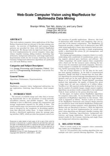
pers were applied in parallel over the particle predictionsand the reducers computed the updated parameters. Experiments were performed on a shared-memory implementationof MapReduce [25].Li et al. [12] developed a landmark classification systemthat uses bag-of-feature [3] vectors and structured SVMs [22]to classify landmarks visually in each photo in a user’s photostream (i.e., temporal sequence of photos). They used adataset of 6.5 million images taken from Flickr and ran experiments using MapReduce. Though the MapReduce algorithm was not described, feature computation was mentioned to be the primary bottleneck.Kennedy et al. [11] explored a method to generate imagetags similar to those found in the ESP game [23] while producing more specific tags. Their approach was to find nearest visual neighbors of photos from different authors andaccept annotations that agree. The nearest neighbor searchwas implemented on MapReduce directly and 19.6 millionFlickr images were used.Yan et al. [24] proposed a scalable concept detection system using robust subspace bagging. The provided MapReduce algorithm consisted of a mapper to train a set ofbase models, a mapper to compute predictions on a validation set, and a reducer to build composite classifiers. Thedataset used consisted of 0.26 million images taken fromvarious sources.3.BACKGROUNDMapReduce [5] builds on the observation that many information processing tasks have the same basic structure: acomputation is applied over a large number of records (e.g.,web pages, nodes in a graph) to generate partial results,which are then aggregated in some fashion. Taking inspiration from higher-order functions in functional programming, MapReduce provides an abstraction for programmerdefined “mappers” (that specify the per-record computation)and “reducers” (that specify result aggregation). Key/valuepairs form the processing primitives. The mapper is applied to every input key/value pair to generate an arbitrarynumber of intermediate key/value pairs. The reducer is applied to all values associated with the same intermediate keyto generate an arbitrary number of final key/value pairs asoutput. This two-stage processing structure is illustrated inFigure 1.Under the MapReduce programming model, a developerneeds only to provide implementations of the mapper andreducer. On top of a distributed file system [8], the executionframework (i.e., “runtime”) transparently handles all otheraspects of execution on clusters ranging from a few to afew thousand cores. It is responsible, among other things,for scheduling (moving code to data), handling faults, andthe large distributed sorting and shuffling problem betweenthe map and reduce phases whereby intermediate key/valuepairs must be grouped by key.As an optimization, MapReduce supports the use of “combiners”, which are similar to reducers except that they operate directly on the output of mappers; one can think ofthem as “mini-reducers”. Combiners operate in isolation oneach node in the cluster and cannot use partial results fromother nodes. Since the output of mappers (i.e., the key/valuepairs) must ultimately be shuffled to the appropriate reducerover a network, combiners allow a programmer to aggregatepartial results, thus reducing network traffic. In cases whereA αB βmappera 1D δmapperb 2c 3combinera 1C γb 2F ζmapperc 6a 5combinerc 6partitionerE εpartitionermapperc 2b 7c 8combinercombinera 5b 7c 2partitionerc 8partitionerShuffle and Sort: aggregate values by keysa1 5b2 7c6 2 8reducerreducerreducerX 5Y 7Z 8Figure 1: Illustration of MapReduce: mappers areapplied to input records, which generate intermediate results that are aggregated by reducers. Localaggregation is accomplished by combiners, and partitioners determines to which reducer intermediatedata is shuffled.an operation is both associative and commutative, reducerscan directly serve as combiners, although in general they arenot interchangeable.The final component of MapReduce is the “partitioner”,which is responsible for dividing up the intermediate keyspace and assigning intermediate key/value pairs to reducers. The default partitioner computes the hash value of thekey and then taking the mod of that value with the numberof reducers. This assigns approximately the same number ofkeys to each reducer.The notation used for algorithms throughout this work isnow described. The job input can come from various sources,though it is commonly stored on a distributed file system.The input key/value pairs are split and distributed amongthe available Map tasks. The Mapper class has a Mapmethod that is called once for each input key/value pair, anoptional Configure method that is called once before thefirst Map call, and an optional Close method that is calledonce after the last Map call. Each Map task maintains aMapper instance. The MapReduce framework distributesMap task keys and associated values among the availableReduce tasks, sorts the Map task outputs by their keys,groups those that have the same key, and presents themto the reducer. The Reducer class has a Reduce methodthat is called once for each unique key and the same optionalConfigure and Close methods as the Mapper class. EachReduce task maintains a Reducer instance.To illustrate the operation of the MapReduce frameworkon a simple task, the following example is provided for counting the number of word occurrences in a series of input documents. Each input is a text document with the key beingthe docid and the value being the document itself. The Mapmethod emits (i.e., adds to the Map task’s output) each wordin the input document as the key and the number 1 as thevalue. There is a key for each unique word and a list of 1’swhich are accumulated by the Reduce method to produce
1: class Mapper2:method Map(docid a, doc d )3:for all term t doc d do4:Emit(term t, count 1)1: class Reducer2:method Reduce(term t, counts [c1 , c2 , . . .])3:sum 04:for all count c counts [c1 , c2 , . . .] do5:sum sum c6:Emit(term t, count sum)Algorithm 1: Example MapReduce algorithm forcomputing word counts given a series of documents.the final word count. The result is emitted (i.e., added tothe Reduce task’s output) with the word as the key and thecount as the value.3.1ImplementationsThere are several implementations of the MapReduce programming model and, while they all maintain the samebasic user abstraction, their capabilities vary considerably.Google’s [5] proprietary implementation is written in C with bindings for other languages. A widely used opensource implementation is Apache Hadoop which is writtenin Java and provides a “streaming” interface to interact withuser code over Unix pipes. Twister [6] is an open-source Javaimplementation and extension of MapReduce optimized foriterative computation. Phoenix [25] is an open-source implementation for shared-memory multiprocessors. In thispaper we use Apache Hadoop’s streaming interface.3.2Design PatternsLin and Dyer [13] introduced design patterns that can beused to simplify and improve the performance of MapReducealgorithms. These design patterns are summarized below asthey are used later in more involved algorithms.3.2.1Order InversionThere are situations where the reducer needs to read thesame or similar input values multiple times to perform thenecessary computation. This often involves using an aggregate statistic for intermediate calculations. An example ofthis occurs when normalizing a set of vectors’ values between [0, 1] when the number of dimensions is larger thanthe number of vectors (e.g., normalizing a video while treating frames as vectors). The mapper emits once for eachdimension with the key being the dimension and the valuebeing a tuple of the vector’s id and the value for the dimension. The reducer can then process the input to findthe minimum and maximum values; however, this requiresreading all of the data, after which we are unable to produce the desired output because only a forward iterator isprovided to the key/value pairs. There is a temptation tobuffer the data in memory and pass over it again; however,this will not scale and eventually the system memory willbe exhausted. A solution is to compute the min/max valuesin the first pass and have another job that computes thefinal output, loading the min/max values as side data froma shared location.Performing the computation in two MapReduce jobs is ascalable solution; however, it can be further improved byusing the order inversion design pattern. The mapper is1: class Mapper2:method Map(vecid i, vector V )3:for all hdim d, val vi vector V do4:t hvecid i, val vi5:Emit(tuple hdim d, flag 0i, tuple t)6:Emit(tuple hdim d, flag 1i, tuple t)1: class Reducer2:method Configure()3:m M p 4:method Reduce(tuple hdim d, flag fi, tuples)5:if p 6 d then# Reset extrema for new dimension6:m 7:M 8:p d9:if f 0 then10:for all tuple hvecid i, val vi tuples do11:UpdateExtrema(val m, val M, val v )12:else13:for all tuple hvecid i, val vi tuples dov m14:v M m15:Emit(vecid i, tuple hdim d, val vi)Algorithm 2: MapReduce algorithm for normalizing vectors using the order inversion design pattern.modified to emit twice for every value with the key andvalue the same as before, except that the key has a flagadded to it that is 0 in one output and 1 in another. Thesort is performed on the dimension first and the flag second.The partitioner is modified to only partition based on thedimension, ignoring the flag so that all data for a specificdimension is sent to the same reducer ordered by the flag.The reducer uses the f lag 0’s to find the min/max values,it can then immediately normalize the f lag 1’s that follow. Instance variables are used to hold state between flagvalues as the grouping is performed on the entire key. Acombiner can be used to decrease the data transfer of thef lag 0’s. Note that the same data transfer, twice whatwas input, is required in both methods for this example;however, order inversion removes the extra job and uses thelocally computed intermediate results which simplifies theimplementation. See Figure 2 for a step-by-step exampleand Algorithm 2 for a concrete implementation. This designpattern is used in Section 4.6 for background subtraction.3.2.2In-Mapper CombiningThe concept of combiners is built into MapReduce to curtail network traffic by performing partial aggregation between the Map and Reduce tasks. The data from the mapper must be sorted for the combiner to operate; however, itis possible to move this computation into the mapper so thatsorting is not required and the amount of data emitted fromthe mapper is decreased. This is accomplished by using thein-mapper combining design pattern which is characterizedby the use of an associative array that is indexed by the output key and the values are aggregated in place. Key/valuepairs will not be emitted for each Map method call, insteadthe final values in the associative array are emitted duringthe Close method. The additional memory required is proportional to the number of unique keys; however, this canbe amended to use constant memory by emitting the least
Map Input(vecid, hdim0 , dim1 i)(0, h9, 6i)Map Output(hdim, f lagi, hvecid, vali)(h0, 0i, h0, 9i)(h0, 1i, h0, 9i)(h1, 0i, h0, 6i)(h1, 1i, h0, 6i)(1, h0, 1i)(h0, 0i, h1, 0i)(h0, 1i, h1, 0i)(h1, 0i, h1, 1i)(h1, 1i, h1, 1i)(2, h1, 0i)(h0, 0i, h2, 1i)(h0, 1i, h2, 1i)(h1, 0i, h2, 0i)(h1, 1i, h2, 0i)(3, h3, 6i)(h0, 0i, h3, 3i)(h0, 1i, h3, 3i)(h1, 0i, h3, 6i)(h1, 1i, h3, 6i)Reduce InputReduce Output(hdim, f lagi, [hvecid0 , val0 i, . . . ]) (vecid, hdim, vali)(h0, 0i, [h0, 9i, h1, 0i, h2, 1i, h3, 3i])(h0, 1i, [h0, 9i, h1, 0i, h2, 1i, h3, 3i]) (0, h0, 1.i)(1, h0, 0.i)(2, h0, 0.1111i)(3, h0, 0.3333i)(h1, 0i, [h0, 6i, h1, 1i, h2, 0i, h3, 6i])(h1, 1i, [h0, 6i, h1, 1i, h2, 0i, h3, 6i]) (0, h1, 1.i)(1, h1, 0.1667i)(2, h1, 0.i)(3, h1, 1.i)Figure 2: Example input and output when normalizing a set of vectors’ values using the order inversiondesign pattern.recently used keys and removing them from the associativearray when a memory limit has been reached. This designpattern is used in Section 4.4 for clustering.3.2.3Value-to-Key ConversionThe MapReduce framework sorts the keys emitted by themapper to group them for the reducer; however, if a taskrequires a primary sort on the key and a secondary sort onfields in the value then you can use the value-to-key conversion design pattern. This design pattern takes part of thevalue and duplicates or moves it to the key to form a newcomposite key. The sort is modified to produced the desiredcomparison priority and ordering. Lastly the partitioner ismodified so that each reducer receives all of the data necessary for the computation (e.g., partition on the originalkey). The primary distinction between order inversion andvalue-to-key conversion is that the former is used to orderintermediate computation, often in the form of an aggregate statistic, while the latter is used to secondary sort thedata. This design pattern is used in Section 4.7 for imageregistration.4.MAPREDUCE & COMPUTER VISIONGenerally, computer vision algorithms operate on one ormore images consisting of pixels and they often have tunable parameters. When deciding how to exploit parallelism,an algorithm designer can generally choose one or more fac-tors along which to divide computation: parameters, images,or pixels. These factors can be thought of as nested foreachloops where one is selected for MapReduce computation withinternal loops residing within the MapReduce Job and external loops corresponding to separate and potentially parallelMapReduce jobs. Computation across algorithm parameters is often embarrassingly parallel (i.e., independent) asare images when an algorithm operates on them independently (e.g., SIFT, face detection).A variety of computer vision algorithms that are applicable to large scale data processing tasks are presented. Thesetasks are desirable to perform on web scale datasets ( 1TBof image data) and are currently limited by the computational capabilities of single machines. These datasets mayconsist of many short videos (e.g., YouTube), long videos(e.g., surveillance footage), consumer images (e.g., Flickr,Facebook), or high resolution images (e.g., satellite imagetiles). The following algorithm descriptions are intended toguide the reader through the process of applying familiarcomputer vision tasks to the MapReduce framework; consequently, implementation details may be omitted for clarityand generality when they do not contribute to the discussion.Moreover, the algorithms are selected to exhibit non-trivialparallel computation and it is assumed that trivially paralleltasks will be performed where applicable in practice.4.1Data RepresentationThe MapReduce architecture depends on a distributedfilesystem as part of its functionality. In the Hadoop implementation, this is the Hadoop Distributed File System(HDFS) and it is based on the Google File System (GFS) [8]used in the original MapReduce implementation [5]. Thesefilesystems are designed around optimal magnetic hard diskaccess patterns involving as few seeks as possible and longstreaming reads. The data is replicated to multiple nodes toimprove availability. A primary optimization made by theMapReduce framework is to avoid remote reads of data toprevent network bandwidth bottlenecks. To accomplish this,the Map tasks are assigned to machines with the necessarydata on local disks when possible.When working with millions of web images, the time toread them in batch is dominated by disk seeks to each fileas the images are often small in size. Moreover, the maximum number of files is limited by the memory capacity ofthe HDFS namenode or the GFS master as the filesystemis kept in memory for efficient access. A portable solutionto this problem is to represent each image and associatedmetadata as a single line in a text file with fields delimited by a special character (e.g., tab). A downside with thismethod is that the raw data must be escaped or encoded toavoid using the field and line delimiters. This representationhas the benefits of being portable between MapReduce implementations, it eliminates the problems with small files,and is efficient to parse; however, the file size is generallylarger than optimal due to the removal of special charactersand ad-hoc metadata encoding introduces complexity. TheHadoop implementation of MapReduce has an input formatcalled SequenceFiles that consists of binary key/value pairs.This format allows us to represent images and arrays in theiroriginal binary form which reduces space requirements andis more computationally efficient to parse; consequently, thisis the representation used in this work.
1: class Mapper2:method Map(metadata d, image i)3:m ParseModelIDs(metadata d )4:p ParsePositiveID(metadata d )5:f ComputeFeature(image i)6:for all id x m do7:if x p then8:Emit(id x, tuple hfeature f, polarity 1 i)9:else10:Emit(id x, tuple hfeature f, polarity 1 i)1: class Reducer2:method Reduce(id m, tuples [t1 , t2 , . . .])3:M InitModel()4:for all tuple hfeature f, polarity pi tuples do5:UpdateModel(feature f, polarity p, model M )6:Emit(id m, model M )Algorithm 3: Algorithm for computing image features (e.g., HoG) and training a classifier (e.g.,SVM) for each object class. The UpdateModelfunction may buffer internally depending on theclassifier.4.2Classifier TrainingWhen classifying objects in a set of images, a standardworkflow is to input images, compute feature descriptors,and train a classifier on the feature descriptors. Using object classification in a surveillance setting as an example,images of pedestrians, cars, and negative examples are usedas input, HoG [4] features are computed, a SVM classifier istrained, and the resulting car and pedestrian classificationmodels are output. To apply this algorithm to the MapReduce framework (see Algorithm 3) the mapper performsthe feature computation in parallel and the features are collected for the reducer where the classifier training is performed. Generalizing to multiple classes, the mapper’s output key is used to specify which model the feature belongsto and emits once for each model. Each reducer receivesthe positive and negative training samples for a set of theclassifiers and trains them sequentially. Optional metadatacan be associated with the feature for use during training(e.g., positive or negative polarity of each feature). In theprovided example, the reducer iteratively adds features tothe classifier; however, this depends on the classifier usedand may require buffering internally.4.3Sliding WindowsOne of the original techniques for object recognition is toconsider a sliding window of an image, compute the classification confidence for the window, and move the windowto another region. After all windows have been considered,thresholding and non-maximum suppression are applied tofind candidate classifications. This technique is computationally expensive as the number of windows considered isO(n) in image pixels; moreover, with the availability of highresolution satellite images the processing time quickly becomes unmanageable for a single machine. To represent thisproblem in MapReduce it is desirable to preprocess the image so that each task has the minimum data necessary whilereducing data redundancy. For example, if the step sizeis such that no pixels are shared between images then thedata can be efficiently represented as an image of each window along with a coordinate offset to relate the original and1: class Mapper2:method Map(offset o, tuple hcoords c, image ii)3:for all coord x c do4:p Classify(image i, coord x )5:if p thresh then6:n Neighbors(offset o, coord x )7:for all coord y n do8:Emit(coord y, tuple hconfidence p, flag 0i)9:Emit(coord x o, tuple hconfidence p, flag 1i)1: class Reducer2:method Reduce(coord n, tuples [t1 , t2 , . . .])3:F P 04:for all tuple hconfidence p, flag fi tuples do5:if P p then6:P p7:F f8:if F 1 then9:Emit(coord n, confidence P )Algorithm 4: ‘Sliding window’ algorithm for objectclassification with non-maximum suppression applied to the output.local image coordinates. However, if dense windows are tobe considered (e.g., one pixel step-size) and the window areais large, then the previous approach makes an inefficient useof storage space. This effect can be reduced by using imagesthat have the necessary data for a number of windows, a coordinate offset, and local image coordinates for each windowin the provided image. As the number of local windows increases the storage size and exploitable parallelism decrease.Algorithm 4 uses the previously described input methodwhere an image, the offset to the original image, and a set oflocal (w.r.t. input image) window coordinates are provided.The classification confidence values are computed in parallelin the mapper and emitted if they are greater than a threshold. To enable non-maximum suppression it is necessary toemit the window confidence K 2 times, where K is the nonmaximum suppression window length. The map output keyis the window coordinates and the value is a tuple of theconfidence and a flag indicating if the confidence belongs tothe window or one of its neighbors. For each window coordinate, the reducer emits the window’s confidence value if itis greater than its neighbors.For simplicity the previous example only considers windows that differ by translation. To generalize the motionto a projective transformation (i.e., translation, scale, rotation, shear, and keystone) the only modification required isto represent each window by its four corner points ratherthan an offset.4.4ClusteringClustering is the process of taking unlabeled points andgrouping them using a distance metric. This is often performed to aid in data analysis and improve computationalefficiency. Clustering is a widely used technique in the fieldsof data mining and computer vision with diverse applications: background subtraction [21], image segmentation [15],and bag-of-features methods [3]. When working with largedatasets, clustering is often necessary to restrict the scopeof higher level analysis while maintaining a reasonable levelof accuracy. A simple and effective clustering method is kmeans, an algorithm that finds the nearest cluster to each
input point and then updates the location of each clusterby taking the arithmetic mean of the points it is nearest to.The algorithm iterates until a stopping condition is met. Toapply this to the MapReduce framework (see Algorithm 5)we find the cluster membership for each point in the mapper, emitting the point’s nearest cluster number as the keyand the point itself as the value. The points are extendedby one dimension and initialized to a value of one to represent the count for cluster normalization. For simplicity, weload the current cluster estimate into memory in the mapper; however, later we will discuss a method that can beused when the clusters are too large to fit into memory. TheMapReduce framework will group the points by their nearestcluster. The reducer sums all of the points and normalizesto produce the updated cluster center, which is emitted asthe value with the key being the cluster number. A ‘driver’program orchestrates the communication of the new clustersto the mapper during the next k-means iteration.In practice the previous implementation will perform poorlyas the entire dataset will be transferred over the networkduring the shuffle phase, resulting in a bottleneck due to thehigh network traffic. We can dramatically improve the performance by observing that the cluster mean computationrequires the sum of all of the points and their cardinality.Addition is associative and commutative which allows us toperform partial aggregation in a combiner that is similar tothe reducer, except that it will not normalize the result. After the combiner runs, it decreases the data sent over thenetwork from O(N ) where N is points to O(KM ) where Kis clusters and M is Map tasks. For the k-means algorithm,Nthe usefulness of the combiner increases as the ratio KMincreases.We can further extend this idea by noting that before thecombiner can run, the mapper output is sorted; however, wecan instead maintain an associative array in the mapper thatholds the partial sums. By using the in-mapper combiningdesign pattern (see Section 3.2.2), the initial algorithm ismodified to not emit during calls to the Map method, andinstead accumulate the partial sums until the Close methodis called after all of the input has been processed (see Algorithm 6). This adds on to the previous optimization bydecreasing the amount of data that is serialized between themapper to the combiner and the time taken to sort the mapper’s output for the combiner. This modification uses up totwice the memory as the original k-means algorithm whilegenerally improving the run-time.To simplify the previous k-means algorithms, we assumedthat there is enough memory to hold the clusters. If thisis not the case then the following extension can be used toperform k-means in three jobs per iteration. We start bypartitioning the clusters into smaller sets that fit into memory. In a map-only job emit the po
Brandyn White, Tom Yeh, Jimmy Lin, and Larry Davis University of Maryland College Park, MD 20742 bwhite@cs.umd.edu ABSTRACT This work explores computer vision applications of the Map-Reduce framework that are relevant to the data mining com-munity. An overview of MapReduce and common design patterns are provided for those with limited MapReduce .