WIXLIB

Online supplement for the manuscript:Analysis of Risk Factors Associated with Renal FunctionTrajectory Over Time: A Comparison of Different StatisticalApproachesKaren Leffondré1, Julie Boucquemont1, Giovanni Tripepi3, Vianda S. Stel4, Georg Heinze2, Daniela Dunkler21.2.3.4.University of Bordeaux, ISPED, Centre INSERM U897-Epidemiology-Biostatistics, Bordeaux, FranceMedical University of Vienna, Center for Medical Statistics, Informatics and Intelligent Systems, Vienna, AustriaCNR-IBIM/IFC, Clinical Epidemiology and Physiopathology of Renal Diseases and Hypertension of Reggio Calabria, Calabria,ItalyAcademic Medical Center, ERA-EDTA Registry, Dept. Medical Informatics, Amsterdam, NetherlandsJuly 2014Table of ContentsAnalyses in SPSS (Version 21) . 2Naive linear regression on invidiual slopes . 2Generalized estimating equations . 8Linear mixed model. 151

Analyses in SPSS (Version 21)The data set can be opened in SPSS:We assume that the reader is familiar with descriptive analyses in SPSS. We directly proceed to outcome analyses ofthis data set, investigating the impact of risk factors age, gender, microalbuminuria at baseline andmacroalbuminuria at baseline on the speed of progression of CKD.Naive linear regression on invidiual slopesThis approach consists of two steps:1) estimation of patient-specific slopes of GFR,2) regression of slopes on risk factors.To estimate patient-specific slopes of GFR, we first ‘split‘ the data by patient ID to have any statistical analyses tofollow carried out on each patient separately. This can be achieved by calling the dialogue Data Split Fileand request Organize output by groups.Move the following three variables into the field Groups based on: Patient identifier [patient]Microalbuminuria at baseline [micro]Macroalbuminuria at baseline [macro]2

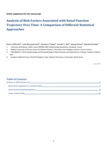
as shown below:Next, we call linear regression by Analyze Regression Linear.:3

Simply move GFR [GFR] into the field labelled Dependent: and Time in years since baseline[time] into the field Independent(s). Next, click on Save.:Here, check Create coefficient statistics and type in a name for the dataset that will later contain theslopes and intercepts per patient (e.g., Slopes).Click on Continue and in the main linear regression dialogue, click on OK.Don’t be surprised, a lot of output – containing the individual regression analysis for each patient - is generated now.Most importantly, a third SPSS window opens, holding the data set with the patient-individual slopes (and somemore information):4

Call Data Select Cases:5

Check the button If condition is satisfied and specify If ROWTYPE “EST“. Then click on OK. Thiswill make sure that we can directly access the slopes per patient which are contained in rows where the variableROWTYPE contains the text EST. Actually, the slopes are in the variable Time in years since baseline[time] since they are the regression coefficients corresponding to this variable in our former regression analysis.The last step consists in calling linear regression (Analyze Regression Linear.) with Time inyears since baseline [time] (a/k/a the slopes) and Microalbuminuria at baseline [micro]and Macroalbuminuria at baseline [macro] as the independent variables:6

The effects of micro- or macroalbuminuria on the speed of progression will then be evaluated:CoefficientsModel1aUnstandardized CoefficientsBStd. ,746,476-3,665,000Microalbuminuria at baseline-3,138Macroalbuminuria at-3,836baselinea. Dependent Variable: Time in years since baseline,722-,319-4,348,000,736-,383-5,214,0007

Generalized estimating equationsAlthough the model is more complex, it is actually much quicker to request a generalized estimating equationsanalysis.Simply go back to the original data set, and undo the splitting per cases (Data Split File):Check Analyze all cases, do not create groups. Click OK.Go to Analyze Generalized linear models Generalized estimating equations.Follow the instructions below:8

9

10

11

Here, click on Options to specify the reference categories for the categorical covariates (called ‘Factors‘ by SPSS):12

Check Descending and click Continue.13

There is nothing to specify at the remaining tabs. Click OK.The parameter estimates of the GEE model will be shown in the output window:Parameter Estimates95% Wald Confidence IntervalParameter(Intercept)[gender 1][gender 0][micro 1][micro 0][macro 1][macro 0]timeage[micro 1] * time[micro 0] * time[macro 1] * time[macro 0] * -,256-1,557a0-1,053a0251,425Std. -,142-,536.,316.Dependent Variable: GFRModel: (Intercept), gender, micro, macro, time, age, micro * time, macro * timea. Set to zero because this parameter is redundant.14Hypothesis TestWald 000,003.,132.

Linear mixed modelThe mixed model can also be obtained using a single menu call. Call Analyze Mixed Models Linear.:Move Patient identifier [patient] into the field Subjects:Click on Continue.Next, specify the dependent an indpendent variables (Factors and Covariates) as below:15

Click on Fixed. to define the way the independent variables are assumed to affect the dependent variable:Move all independent variables, as well as the interaction of micro and macro with time into the Model field. ClickContinue.Next, click Random. to define the random effects.16

Move time into the Model field and check Include intercept. Select as covariance type CompoundSymmetry: Heterogenous. (Some other heterogenous covariance types with nonzero off-diagonals will alsolead to same result here.) Move Patient identifier [patient] into Combinations.Click Continue.Click on Estimation and select Maximum likelihood (ML).17

Click on Statistics and select Parameter estimates, and Covariances of random effects.18

Finally click on OK.In the results table (below), you will notice that SPSS will use the first level of each factor as the reference category,without offering any options to change this. This does not change the interpretation of the main results.Estimates of Fixed EffectsParameterEstimateStd. ErrordfIntercept35,8134134,176224198,483[gender 0]2,6184761,677175197,213b[gender 1]00.[micro 0]18,3994861,871395194,979b[micro 1]00.[macro 0]26,5647161,892764198,486b[macro 197,213[micro 0] * time2,920882,636944177,043b[micro 1] * time00.[macro 0] * time3,091009,668498189,621b[macro 1] * time00.a. Dependent Variable: GFR.b. This parameter is set to zero because it is 00.95% Confidence IntervalLower BoundUpper 8787-,1860011,6639024,177861.1,7723624,409656.

Analyses in SPSS (Version 21) The data set can be opened in SPSS: We assume that the reader is familiar with descriptive analyses in SPSS. We directly proceed to outcome analyses of this data set, investigating the impact of risk factors age, gender, microalbuminuria at baseline and macroalbuminuria at baseline on the speed of progression of CKD.