WIXLIB

3Yet single-stage models are insufficient to test the double-trigger hypothesis. In the context of thedouble-trigger hypothesis, entering arrears can best be viewed as the first step in the process – thatof experiencing an ability-to-pay shock. The second step, proceeding to foreclosure based on a loan’sequity position, is untested in these studies. Moreover, many loans that enter arrears willsubsequently cure. It is common for papers to argue that examining entries to 60 or 90 dayarrears is sufficient to understand defaults, but these papers are often estimated using data forsubprime loans during the global financial crisis, for which foreclosure was more common(e.g. Bhutta et al 2017). Adelino, Gerardi and Willen (2013) show that up to 70 per cent of loansthat entered 60 day arrears self-cure in a more representative dataset of loans (although thispercentage fell during the financial crisis). Conversely, papers that study foreclosure alone miss themany loans that may enter arrears but subsequently cure (e.g. Bajari, Chu and Park 2008).The set of papers that study the transition from arrears to foreclosure is relatively small. Thesestudies typically examine either foreclosure mitigation policies or the role of securitisation, ratherthan the double-trigger hypothesis (Piskorski, Seru and Vig 2010; Kruger 2018). An exception isAmbrose and Capone (1998), who similarly argue that foreclosure is a separate process to aborrower entering arrears. They estimate a multinomial logit for whether borrowers in arrears go onto foreclose or to cure. Do, Rösch and Scheule (2020) examine the dollar value of losses given thatloans have defaulted; they find that borrower liquidity constraints and negative equity affect whetherloans cure and negative equity also increases the dollar value of losses.A problem commonly encountered in the empirical literature is measurement error. While moststudies provide good estimates of a loan’s equity (utilising loan-to-valuation ratios, indexed forchanges in regional housing prices), they frequently fail to identify individual shocks to a borrower’sability to repay. 1 Instead, papers often rely on regional economic data, such as regionalunemployment rates, as a proxy for individual shocks. Gyourko and Tracy (2014) find that theattenuation bias from using regional variables may understate the true effect of unemployment bya factor of 100. With a loan-level dataset, I have access to borrower and loan characteristics, butsimilarly resort to more aggregated proxies such as the regional unemployment rate wherenecessary.As noted above, studies of the determinants of mortgage default in Australia have been scarce. Readet al (2014) use a hazard model framework and find that loans with riskier characteristics and higherservicing costs are more likely to enter arrears. However, very few loans in their sample havenegative equity, preventing a thorough analysis of the implications of negative equity. Likewise, alack of foreclosures in their dataset prohibits their examination. In a survey of borrowers thatunderwent foreclosure proceedings, Berry, Dalton and Nelson (2010) find that a combination offactors tend to be involved in foreclosures, with the most common initial causes being the loss ofincome, high servicing costs and illness. However, the sample size of this survey is low, partlyreflecting low foreclosure rates in Australia. Kearns (2019) examines developments in aggregatearrears rates in Australia and concludes that the interaction of weak income growth, housing pricefalls and rising unemployment in some regions, particularly mining-exposed regions, havecontributed to an increase in arrears rates in recent years.1There are some exceptions. Elul et al (2010) use borrowers’ credit card data as a proxy for liquidity constraints. Gerardiet al (2018) highlight the importance of unemployment and disability shocks using household-level survey data.

4Empirical research examining the implications of regional stress events for mortgage default hasbeen limited, but Gerardi et al (2008) show that this can be a fruitful exercise. When predictingdefaults during the early stages of the financial crisis, they show that models estimated using dataon the early 1990s Massachusetts recession and housing downturn outperform models estimatedusing a broader dataset of US loans from 2000 to 2004. This is attributed to the lack of loans withnegative equity through the latter period and highlights the need for an appropriate sample period.An earlier study by Deng, Quigley and Van Order (2000) compares models estimated for loans inCalifornia and Texas through 1976 to 1992, when California experienced strong housing price growthand Texas was affected by an oil price shock and housing price declines. They find that coefficientstend to be larger for the Texan loans and conclude that unobservable differences between theregions may be important; these differences could include nonlinearities associated with the stressevent.A number of empirical studies examine the influence of institutions and legal systems on mortgagedefault, such as the effect of full recourse or judicial foreclosure (Mian, Sufi and Trebbi 2015; Linnand Lyons 2019). Australia has full recourse loans, which raises the cost of defaulting for borrowersthat have other assets. Research comparing defaults across US states finds that full recourse actsas a deterrent to defaults, particularly strategic defaults, and raises the amount of negative equitythat is required for a borrower to default by 20 to 30 percentage points (Ghent and Kudlyak 2011;Bhutta et al 2017). By raising the cost of foreclosure for borrowers with multiple assets, full recoursemay cause borrowers to rationally attempt to avoid foreclosure even when their mortgage is deeplyin negative equity. For sufficiently large values of negative equity, however, foreclosure will still bethe rational response even in the presence of full recourse.3.Data Description3.1Securitisation DatasetThe Reserve Bank of Australia (RBA) accepts residential mortgage-backed securities (RMBS) ascollateral in its domestic market operations. Since June 2015, collateral eligibility has requireddetailed information about the security and its underlying assets to be provided to the RBA. Thesedata, submitted on a monthly basis, form the Securitisation Dataset and as at June 2019 containeddetails on approximately 1.7 million residential mortgages with a total value of around 400 billion.This represents roughly one-quarter of the total value of housing loans in Australia and includesmortgages from most lenders. Around 120 data fields are collected for each loan, including loancharacteristics, borrower characteristics and details on the property underlying the mortgage. Suchgranular and timely data are not readily available from other sources.The loans are not, however, representative of the entire mortgage market across all of its dimensions(see Fernandes and Jones (2018) for more details). This partly reflects the securitisation process.For example, there can be lags between loan origination and loan securitisation; we typically cannotobserve the first months of a loan’s lifetime and recent loans are under-represented in the dataset.Issuers of securitisations may also face incentives to disproportionately select certain types of loans,such as through the credit rating agencies’ ratings criteria. For example, the Securitisation Datasetcontains a lower share of loans with original loan-to-valuation ratios (LVRs) above 80 per cent thanthe broader mortgage market, as well as a lower share of fixed-rate mortgages (Fernandes andJones 2018). Issuers of some open pool self-securitisations also remove loans that enter arrears

5from the pool; to avoid selection effects, I remove deals that exhibit this behaviour from my analysis.2While it appears unlikely that these differences would have a large effect on the model coefficients,aggregate arrears rates may differ to that of the broader mortgage market due to thesecompositional differences.I use observations for 2.8 million individual loans that were reported in the Securitisation Dataset atany point between July 2015 and June 2019. Around 45,000 of these loans entered 90 day arrearsat some point during this period (around 1.5 per cent of loans) and around 3,000 loans proceededto foreclosure. Further details on the construction of the samples used for the models are providedin Section 5. Summary statistics and variable definitions are provided in Appendix A.3.2Indexed Loan-to-valuation RatiosI calculate indexed LVRs to estimate the equity position of mortgages, as per Equation (1).3 Tocapture changes in housing prices, I use regional housing price indices to update property valuations.This approach is standard within the literature, but does introduce some measurement error – itcannot account for changes to the quality of the property and may not be precise enough to accountfor highly localised changes in prices. It also does not account for borrowers’ price expectations.Indexed LVR Consolidated scheduled balanceMost recent property valuation 1 subsequent regional house price growth (1)Hedonic regional housing price indices are sourced from CoreLogic. These data are available forStatistical Area Level 3 (SA3) regions (there are around 350 SA3 regions in Australia, each comprisingbetween 20,000 and 130,000 residents). As at June 2019, housing prices had declined from theirpeaks in most regions (by around 8 per cent on average), but had fallen by as much as 70 per centin some mining-exposed regions (Figure 1).A loan is defined as having negative equity if its indexed LVR is above 100 (i.e. the estimated valueof the property has fallen below the amount owing on the mortgage). The incidence of negativeequity has been fairly rare in Australia, at around 4 per cent of the loans in the dataset in 2019. 4These loans were mostly located in the mining-exposed regions of Western Australia, Queenslandand the Northern Territory, and many were originated between 2012 and 2016 (Figure 2; seeRBA (2019) for further details). Many of these loans were located in metropolitan Perth and Darwin.Note that I classify SA3 regions as mining-exposed if they contain at least two coal, copper or ironore mines or if at least 3 per cent of the labour force is employed in the mining industry.234Self-securitisations are held entirely by the originating banks for use as collateral in the RBA’s market operations. Manyof these deals have ‘open’, or ‘revolving’, pools; that is, loans can be added or removed from the pool.The scheduled loan balance differs from the current loan balance by abstracting from any additional repaymentspreviously made, including those in redraw and offset accounts, which a borrower would be able to draw upon priorto defaulting. The calculation does not take into account additional debts, such as credit card debts or debts withother lenders.This figure is higher than estimates in RBA (2019) due to the use of scheduled balances in the LVR calculation.Estimates from the Securitisation Dataset may understate the incidence of negative equity due to the skew towardsloans with lower LVRs at origination, or overstate it due to the prevalence of newer loans in the dataset.

6Figure 1: Selected Regional Housing Price IndicesJanuary 2008 100indexMetro areasMining-exposed regionsSydney CityindexEast Pilbara150150MelbourneCity10050100Brisbane InnerDarwin CityPerth CityBowen Basin50West Pilbara02009Sources:20142009020192014Author’s calculations; CoreLogic dataFigure 2: Share of Securitised Mortgages with Negative EquityBalance-weighted share of securitised loans, June and ACTSAABS; Author’s calculations; CoreLogic data; RBA; Securitisation SystemQldWAand NT0

7The extent of negative equity has also been greater in mining-exposed regions, particularly in nonmetropolitan regions (Figure 3). Since the risk of foreclosure may increase nonlinearly with theextent of negative equity, regional mining areas play an important role in identifying the relationshipbetween negative equity and default risk.Figure 3: Distribution of Indexed LVRsBalance-weighted share of securitised loans, June 2019%9Positive equity633%Non-mining regions99663300255075100125Indexed LVR – %Metro3.39Negative equity6%Sources:%Mining-exposed regions1501750200Non-metroABS; Author’s calculations; CoreLogic data; RBA; Securitisation SystemCensus DataRegional economic data are sourced from the ABS Census. Key among these is the regionalunemployment rate. I use a version of the unemployment rate that adjusts for internal migration; itrecords the unemployment rate of working-age individuals in 2016, based on the SA3 region in whichthey lived at the previous census in 2011. Adjusting for internal migration is important in the contextof the winding down of the mining investment boom, as many unemployed workers had migratedfrom mining regions to other areas in search of employment, particularly to capital cities. Unadjustedregional unemployment rates are a poor proxy for the true probability that home owners frommining-exposed areas experienced unemployment.54.Stylised FactsThe stylised facts in this section are consistent with the double-trigger hypothesis; arrears rates havea positive relationship with regional unemployment, and foreclosure rates are higher for loans withnegative equity. But econometric modelling is still required to separately identify the two distinct5Using the unadjusted unemployment rate in my model produced smaller coefficients that were generally notstatistically significant.

8triggers, not least because the regional incidence of unemployment and negative equity arecorrelated.4.1Entries to Arrears are Correlated with Regional Unemployment RatesAt the region level, entries to 90 day arrears are positively correlated with unemployment rates;both tend to be higher in mining-exposed regions (Figure 4). The regions with the highest shares ofloans entering arrears are ‘Outback Western Australia’ (particularly the Pilbara), ‘OutbackQueensland’ and Mackay.Quarterly entries to 90 day arrears – %Figure 4: Regional Arrears and UnemploymentLoans originated since xposed regionsNon-mining regions6912Unemployment rate – %15Entries to arrears are averaged over 2015–19; 2016 unemployment rate by usual place of residence in 2011; SA4 regionsABS; Author’s calculations; RBA; Securitisation SystemLoans with Negative Equity are More Likely to Transition to ForeclosureTransitions of loans from arrears, and the time they take to transition, are a function of bothborrowers’ and lenders’ actions. In Australia, lenders issue borrowers with a notice of default oncea loan enters 90 day arrears (ASIC nd). Lenders may commence legal action to repossess theproperty if the borrower does not become fully current on their mortgage payments within the noticeperiod, which is at least 30 days. The loan is defined as being in foreclosure once the ownership ofthe property has been transferred to the lender, and the lender will then make arrangements to sellthe property. The lender may seek a court judgement for recourse to the borrower’s other assets ifthe sale price of the property is insufficient to cover the amount owing plus foreclosure costs.Under Australian consumer credit protection regulations, borrowers may submit a hardshipapplication to their lender following the receipt of a notice of default, outlining why they areexperiencing repayment difficulties, how long they expect their financial difficulties to continue and

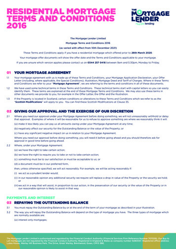
9how much they can afford to repay. Lenders are required to consider hardship variations wherecases are deemed to be genuine and meet certain requirements, and to provide alternatives suchas repayment holidays or an extension of the loan term. Lenders will also typically delay legalproceedings when borrowers provide evidence that they are in the process of selling their property.The transitions of loans from arrears are highly correlated with the loans’ equity positions as at thetime they entered arrears (Figure 5). Most loans with positive equity eventually cure (defined asbecoming fully current on their scheduled payments) or are fully repaid (i.e. resolved through theborrower selling the property or refinancing). On the other hand, the share of loans that go on toforeclose is increasing in the degree of negative equity, as the borrower cannot profitably sell theirproperty to avoid foreclosure and the probability that the value of negative equity exceeds the costof foreclosure increases with the extent of negative equity. Loans in arrears that are deeply innegative equity have around a 50 per cent probability of eventually transitioning to foreclosure.Some readers may be surprised that this share is not higher; perceived foreclosure costs, fullrecourse to other assets (including other properties) and borrower expectations of a future housingprice recovery may be contributing factors.6Figure 5: Transitions from 90 Day ArrearsShare of loans that have transitioned from first arrears event150 ndexed LVRForeclosureNote:Sources:6RepaidCuredFinal status of loans (excludes loans that remained in arrears at last observation)Author’s calculations; CoreLogic data; RBA; Securitisation SystemThis figure is based on the indexed LVR at the point of entering arrears; results are little changed after accounting forsubsequent changes to housing prices. It is possible that borrowers with substantial negative equity may still chooseto cure if they expect housing prices to subsequently recover.

10Although foreclosure rates are higher for loans with high LVRs, by number the majority of foreclosedloans appear to have slightly positive equity when they enter arrears. Several factors may explainthis, including that equity may have been mismeasured. Mismeasurement could occur if the loanbalance does not capture all debts (such as subsequent accumulated balances in arrears

determinants is important for understanding the risks associated with mortgage defaults, and how these can be mitigated. Yet there have been few studies of the determinants of mortgage defaults in Australia, likely reflecting relatively low default rates and the absence of widespread stress events for periods when detailed data has been available.