WIXLIB

A&A 662, A35 (2022)four Unit Telescope (UT) MULTIMR42 mode (R 75 000 with4 2 binning), ESPRESSO has already proven to be effectivein using QALs to constrain our understanding of the Universe(Cooke et al. 2020; Welsh et al. 2020). However, these observations require all four UTs simultaneously, and the collectionof light from MULTIMR42 mode means a reduction of R from 137 000 to 75 000, a resolution UVES can obtain withoutexcessive slit losses in average Paranal atmospheric conditions.As of Period P108, ESPRESSO supports a single UT mode with4 2 binning (HR42 mode). This mode is designed to reduceread-out noise while maintaining a high spectral resolving power(R 137 000), and it is ideal for observing faint targets such asQSOs.In this paper, we present the results from a pilot programmeto test the ability of ESPRESSO’s HR42 mode to analyse thechemical contents of a DLA seen along a quasar sightline andcompare the performance of ESPRESSO HR42 mode to thetypical observing set-up used for UVES.2. Target selection, observations, and datareductionThe target, QSO J0003 2603 (right ascension 00 h030 22.95300 ,declination 26 030 18.30700 , and redshift zem 4.01), was chosen as it is (i) sufficiently bright for the ESPRESSO autoguidingsystem (AB magnitude R 18.5 mag), (ii) known to host anintervening metal-poor ([M/H] 2) DLA absorber along theline of sight (redshift zabs 3.39), and it (iii) has archival UVESobservations allowing a direct comparison between instruments(Molaro et al. 2000; Levshakov et al. 2000).The ESPRESSO observations were carried out on October 22021 on UT2 at Paranal (Programme ID 60.A-9801(W)). Foursequential 60-minute on-target exposures were taken. The observations were made in average seeing conditions ( 0.7700 ; imagequality at 5000 Å of 0.8500 ) across the four hours of observations at an average airmass of 1.05. The data were reducedwith the default settings of the ESPRESSO ESO-reflex pipeline(version 2.3.3; Pepe et al. 2021; Freudling et al. 2013) and postprocessed with the ESPRESSO data analysis software (hereafterDAS; version 1.3.3; Cupani et al. 2019; Pepe et al. 2021). Whilewe used the sky-subtracted data in this paper to avoid skylinecontribution, we point out that the S/N is marginally better in thespectrum without sky subtraction. The S/N (in units of pixel 1 ; 1 km s 1 per pixel) is 20 within the Lyα forest and 30beyond the Lyα emission line of the quasar.The quoted resolving power of the HR42 mode, based onthe ThAr arc calibrations taken by ESO, is R 131 000. Tocompare what was achieved by our data, we quantified R usingthe telluric lines from two different methods. We first assumedthat the measured full width at half maximum (FWHM) of aweak, unresolved telluric line is equal to the FWHM of theresolution element (FWHMres ); the measured FWHMres of thetelluric line at 7685 Å within the median-combined spectrumis 2.269 0.292 km s 1 (corresponding to R 132 100). However, this method assumes that telluric lines are unresolved byESPRESSO, which is not necessarily true given the high spectral resolution of the HR42 mode. To confirm the specific telluricline was unresolved and to obtain a second, independent measurement of the resolving power, we fitted the telluric linesusing using MOLECFIT (Smette et al. 2015), which providesboth an estimate of FWHMres as well as the intrinsic FWHMof the telluric line based on a model atmosphere at the timeof observations. Taking the mean value from each individualexposure, the MOLECFIT-estimated intrinsic FWHM of theA35, page 2 of 8telluric line at 7685 Å is 1.480 0.050 km s 1 and FWHMres 2.193 0.050 km s 1 (R 136 700). It is clear from the resultsof MOLECFIT that the telluric line at 7685 Å is marginally unresolved within our data set. However, we caution that dependingon the airmass and atmospheric conditions at time of observations, the telluric lines may be resolvable by ESPRESSO’s HRmode and will not provide an accurate estimate of the resolvingpower of the instrument. We adopt R 136 700 from MOLECFITas the best estimate of the resolving power of the HR42 mode.The comparison archival UVES data used 4.5 h of on-targetexposures and was combined and continuum normalised by theUVES Spectral Quasar Absorption Database team (SQUAD;Murphy et al. 2019). Observations were executed during thecommissioning of UVES (Programme ID 60.A-9022(A); slitwidth 0.900 with the DIC2 437 860 instrument setup) andwere observed at a similar airmass and at various seeing measurements (from 0.3400 to 2.400 ; mean of 1.000 at 5000 Å)across two nights. Using unresolved telluric lines within thedata, the obtained FWHM of the spectral resolution element isFWHMres 5.981 0.126 km s 1 (R 50 100; archival R measurements from ThAr arc lines obtained R 47 900). The UVESpixel size is 2.5 km s 1 . The S/N per pixel is 2 (alternatively, 1.33 per Å) larger within the UVES spectrum relativeto that of ESPRESSO (Fig. 1). Once accounting for the difference in pixel size between the two instruments, the S/N ofUVES becomes significantly better than that of ESPRESSO at.5000 Å.3. Results3.1. Comparison with the ESO Exposure Time CalculatorFigure 1 shows the observed S/N (red line) across the entirespectrum compared to what was estimated using version P109 ofthe ESPRESSO Exposure Time Calculator (ETC; black points).The ETC S/N estimates were computed assuming a 0.8400 imagequality, the average airmass through the observations (1.05), anda fractional lunar illumination of FLI 0.0 as the moon was notvisible during observations. The S/N estimated by the ETC isconsistently 1.3 higher across the entire wavelength range.However, we point out that the ETC solely includes emissionfrom the QSO continuum and not absorption lines observedtowards QSO J0003 2603 (particularly those of the Lyα forest; 6202 Å), thus leading to an overestimation of the S/N. Thisis particularly demonstrated by the presence of the strong Lyαabsorption from the DLA at zabs 3.39 ( 5300 Å in red line ofFig. 1). Using only pixels of the observed ESPRESSO spectrumwith predominantly quasar continuum flux near the centres ofESPRESSO’s spectral orders, the observed S/N is only 1.15 smaller than the ETC predicts.To obtain a near-equivalent spectrum with UVES (i.e., R 110 000) and wavelength coverage from 3800 Å to 7880 Å),one would need to observe with two UVES settings (e.g. DIC1390 580 and DIC2 437 760) and with slit widths of 0.300 . Thecyan points in Fig. 1 show the ETC-predicted S/N for the UVESspectrum using these two settings and a 0.300 slit width, with anexposure time of four hours per setting under the same observing conditions as the ESPRESSO observations. The S/N of thecyan points is 2 higher per pixel than what is observed withESPRESSO for two reasons. First, as there is a wavelengthoverlap between the two UVES settings, there is an increasein the S/N in the wavelength ranges 3760–4480 Å, 4770–4960 Å, and 5700–6780 Å. Secondly, the UVES unbinned pixel

Signal-noise ratio(pixel 1)T. A. M. Berg et al.: ESPRESSO HR42 performance for observing quasars8060QSO LyESPRESSOESPRESSO ETCUVES (0.9" slit)UVES ETC (0.3" slit)402004000 4500 5000 5500 6000 6500 7000 7500(Å)Fig. 1. S/N (per pixel; 1 km s 1 per pixel) of the observed ESPRESSO spectrum (solid red line) and ETC-estimated values based on a QSOemission template (black circles). The observed spectrum S/N is estimated as the measured flux divided by the standard deviation from the errorspectrum. We note that the red line is smoothed by taking the median S/N within a wavelength bin of the same size as the average space betweenETC points. For reference, the vertical grey line denotes the Lyα emission line of the observed QSO. The S/N from the ETC consistently .20%larger than measured in the observations. For reference, the smoothed S/N from the comparison UVES data ( 2.5 km s 1 per pixel) is shown asthe blue dotted line. Due to the gaps in the UVES data wavelength coverage, the observed UVES data do not cover the Lyα emission of the QSO.Additionally, the small cyan dots represent the combined ETC estimate for UVES data taken with two UVES settings, with each setting using a0.300 slit (near equivalent R) with the same exposure time per setting (i.e. doubled observing time) and observing conditions as the ESPRESSOdata.3.2. Characterisation of the intervening absorber withESPRESSOBy simultaneously fitting the continuum and a Voigt profile toboth the Lyα and Lyβ lines, the measured H I column density of the intervening absorber towards QSO J0003 2603 islog N(H I) 21.35 0.12 at zabs 3.3901. The measured H Icolumn density is consistent with previous measurements (Luet al. 1996). The Voigt profile fit to the Lyα absorption line isshown in Fig. 2.Additionally, Voigt profile fitting was done for absorptionlines of key metal species (C IV, N I, Si II, Al II, Fe II, Ni II). Wenote that in the analysis of the UVES data done by Molaro et al.(2000) there was sufficient S/N in the Lyα forest ( 10 pixel 1 ) todetect the O I lines λ 925 Å and 950 Å ( 4115 Å in the observedframe). However, the efficiency of ESPRESSO at blue wavelengths is too poor to be able to accurately model the continuum1.0Normalized fluxsampling of the resolution element of this setup is 1.39 pixelsper element in the blue and 1.94 pixels in the red. Not only doesthis pixel size lead to under-sampling in the spectral direction,but also it results in an increase in S/N per pixel of 1.18–1.39 compared to ESPRESSO. Thus, the expected ratio of the S/Nbetween UVES and ESPRESSO – after accounting for the doubled exposure time in overlapping regions of the two UVESsettings and the resolution element size – is between 1.18 and1.97, and this explains the majority of the discrepancy betweenthe red curve and cyan points of Fig. 1. While ESPRESSO isexpected to be as efficient as UVES with a 0.300 slit to obtaina R 100 000 spectrum, ESPRESSO is able to obtain fullwavelength coverage (3800–7880 Å) in a single setup whilstNyquist sampling the spectral resolution element, making theHR42 mode more efficient in terms of observing time required.0.80.60.40.20.010000500005000Relative velocity (km s 1)10000Fig. 2. Best-fit Voigt profile of Lyα (cyan line) to the continuumnormalised ESPRESSO data (black line) for the absorption seen atzabs 3.3901. The best-fitting H I column density is log N(H I) 21.35 0.12. The shaded cyan region denotes the range of profiles fromthe error on log N(H I).within the Lyα forest, although it is possible to see evidence ofsaturation of the O I λ929 Å and 950 Å lines. Unfortunately, thewavelength coverage of ESPRESSO does not include coverageof Cr II and Zn II at the redshift of the DLA.The fitting was done using the code ALIS1 , which uses aχ2 minimisation to simultaneously fit the continuum and profile components from a list of starting redshifts (z), the turbulentcomponent of the Doppler broadening parameters (bturb ), gastemperature (T gas ), and column densities (N; in units atomscm 2 ) for each ionic species. A Gaussian FWHM of 2.193 km s 11https://github.com/rcooke-ast/ALISA35, page 3 of 8

A&A 662, A35 (2022)Table 1. Component Voigt profile fits for low ions.z v (km s 1 )bturb (km s 1 )123453.3895123.3898923.3900563.3901883.390481 42 16 54248.1 0.274.3 0.095.1 0.125.1 0.0913.7 0.6812343.3895113.3899493.3901303.390505 42 120268.4 0.397.0 0.116.5 0.0915.4 1.17Comp.log N(N I)ESPRESSO13.25 0.175.13.30 0.082 13.71 0.06814.26 0.021 14.56 0.19814.32 0.019 14.73 0.053.13.29 0.028.UVESis used as the ESPRESSO line spread function in the fittingprocedure. As the HR42 mode provides sufficient resolution topossibly constrain gas temperature (Narayanan et al. 2006), werepeated the fitting process by including T gas as a free parameter per absorption component. Despite having a range of ionsof varying atomic mass, many lines in this system are blendedor saturated, preventing a realistic constraint on T gas ; includingT gas as a free parameter in the model suggests a purely turbulentmedium. In order to obtain an accurate measure of the columndensities for all components of each ion, we elect to assumeT gas 10 000 K, which is a typical temperature of metal-poorDLAs (Cooke et al. 2015), rather than separately fitting a singleDoppler parameter to each ion’s component. While assuming asingle T gas may not provide accurate measurements of bturb foreach component, the Voigt profile fitting procedure will be moreprecise as the fit is constrained by more data (i.e. multiple ionsprobing the same bturb ) and effects from atomic mass are properlyaccounted for. As a result, this will reduce the overall errors inboth the Doppler parameter and log N. Furthermore, by derivingbturb for each component, the fitting also breaks the degeneracybetween the Doppler parameter and column density for saturatedlines, enabling a measurement of the column density for Si IIand Al II. We note that repeating the fitting procedure with aT gas within the range of DLA values (i.e. from 1000–100 000 K)has little effect on the derived column densities, which remainconsistent with the assumed T gas 10 000 K column densities.By assuming a fixed T gas , the errors derived from fitting bturbencapsulate the errors on the total Doppler parameter. The highions (i.e. C IV) and low ions (N I, Si II, Al II, Fe II, and Ni II)were fitted separately, and assuming that the z of each component of the low ions’ velocity profile are the same across allspecies. Given the level of blending and saturation for many ofthese lines, which introduces model degeneracies while fittingall lines simultaneously, the velocity profiles were fitted in several iterations to constrain individual components free of thesedegeneracies. First, the strongest components at 0 km s 1 werefitted using the unsaturated Fe II λ1611 Å and the two redmostlines of the N I λ1134 Å triplet (λ1134.4 and 1135.0 Å) to fixbturb , z, and N(Fe II) for these two components that cannot be easily determined from the saturated lines. The redshifts of the restof the profile (five components total) were then fixed using theunblended Fe II λ1608 Å, before running the fit on the remaininglines to determine the remaining parameters. These ALIS models were subsequently cross-checked with the ESPRESSO DAS;the results of the two methods are in agreement within the uncertainties. The best-fit absorption profile parameters are presentedA35, page 4 of 8log N(Si II).14.96 0.00914.59 0.018.log N(Al II)log N(Fe II)log N(Ni II)12.14 0.01712.30 0.01713.17 0.06812.86 0.03012.06 0.02413.38 0.05813.59 0.01514.57 0.02614.07 0.01512.97 0.06212.59 0.271.13.14 0.04512.92 0.05211.96 0.91112.09 0.05412.79 0.01213.29 0.02911.92 0.03513.40 0.01913.99 0.00814.63 0.01812.82 0.086.in the top of Table 1, while the velocity profiles and their corresponding fits are shown in the two leftmost columns of Fig. 3.For reference, the velocity of each component relative to zabs ( v)is tabulated in Table 1.Similarly, we applied the same profile fitting method to thelow ions in the UVES data (assuming an instrumental resolution element of 5.981 km s 1 ; right column of Fig. 3; bottomof Table 1) and detected only four components. Components 2,3, and 4 of the ESPRESSO fit (Table 1) are separated by 20 km s 1 , and all three components have a bturb below theresolving power of the 0.900 UVES set-up (FWHM 6.4 km s 1 ).As component 2 is weaker than the other two components, theasymmetry in the line profile can be detected within the UVESdata, while components 3 and 4 cannot be distinguished. Thus, asa result of the 3 larger spectral resolving power of the HR42mode, more components with small bturb can be detected withESPRESSO despite the modest S/N.Given the strength of the Si II λ1526 line in the ESPRESSOdata, we point out that there appears to be an artefact in theUVES data near the Si II λ1808 Å line. The profile shape appearsshifted blueward in velocity space ( 5 km s 1 ) with reference to the other lines (right column of Fig. 3), leading to apoor fit using the fixed redshift and bturb from the Al II andFe II lines. The resulting log N(Si II) is severely inconsistentwith the ESPRESSO value. Fitting a separate, independent, twocomponent profile to the Si II 1808 line results in a total columndensity estimate of log N(Si II) 15.65, which is inconsistentwith the sum of the components 2, 3, and 4 of the equivalent absorption feature in the ESPRESSO data (log N(Si II) 15.07 0.16).The same fitting method was also applied to the C IV doubletvelocity profiles (Fig. 4). The complexity of the C IV absorptionprofile combined with either the modest S/N of the ESPRESSOor the resolution of the UVES data leads to a degenerate parameter space, requiring anywhere between ten and 16 componentsto provide a satisfactory fit. Many of the additional components beyond the initial ten are much weaker, with either thecolumn density being several orders of magnitude smaller thanthe total value and thus consistent with the noise, or the profileshapes being shallow and/or broad and potentially accountedfor by modifying the continuum fit. In many cases, these additional components contribute minimally to the total columndensity. For the UVES data, the minimum ten components weresufficient to reproduce the absorption profile (right column ofFig. 4). As with the low ion profile, the ESPRESSO data isable to resolve an additional two components (at v 22 and

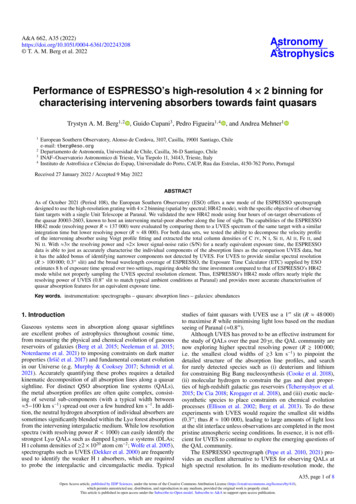
T. A. M. Berg et al.: ESPRESSO HR42 performance for observing quasarsESPRESSO1.0ESPRESSOUVES0.50.01.0NI 1134bFeII 1608SiII 1808NI 1134cFeII 1611AlII 1670SiII 1526NiII 1703FeII 1608AlII 1670NiII 1709FeII 1611FeII 1144NiII 1751Relative 00Relative velocity (km s 1)Fig. 3. Velocity profiles of key low-ionisation absorption lines (labelled in the bottom right corner of each panel) detected within the continuumnormalised data (black lines) of QSO J0003 2603. The panels of the left two columns of the figure denote data from ESPRESSO, while therightmost column shows the absorption lines of the UVES data. The solid magenta curve denotes the complete Voigt profile fitted to the data,while the red dashed lines denote the components that constitute the fit. Overplotted in cyan are the blended components. Although the profile forN I λ1134.1 Å was not fit due uncertain continuum blueward of the line, the expected profile shape based on the fits of the other two triplet lines(λ1134.4 Å [1134b] and λ1135.0 Å [1134c]) is shown in the N I 1134b panel at 70 km s 1 .57 km s 1 ; left column of Fig. 4). The properties of each component for both data sets are tabulated in Table 2. The recoveredtotal column density of C IV from UVES and ESPRESSO areequivalent.3.3. Comparison of DLA properties between ESPRESSOand UVESTable 3 provides the total column densities derived from theESPRESSO and UVES Voigt profile fitting analysis. Errors onthe total column densities include continuum fitting errors. Comparing the total column densities derived from ESPRESSO withthose from UVES (both from the analysis in this paper andMolaro et al. 2000), all values are consistent. We note thatMolaro et al. (2000) only fitted the low ions’ absorption profileswith a single component, thus excluding the weak components 1,2, and 5 from the ESPRESSO fit (Table 1; components 1 and4 from UVES). However, we emphasise that these three weakcomponents contribute minimally to the total column densities, and our derived total column densities are consistent withMolaro et al. (2000). Thus, while in Table 3 we conservativelyassume log N(Si II) is a lower limit as components 1 and 2 areseverely blended, it is likely that they have little contribution tothe total column density of Si II. Ignoring these missing components would imply a total log N(Si II) 14.99 0.217 fromESPRESSO.A35, page 5 of 8

A&A 662, A35 (2022)ESPRESSORelative flux1.0UVES0.5CIV 15480.01.0CIV 15480.50.0200CIV 15500100 200 100 1 0Relative velocity (km s )100CIV 1550100Fig. 4. Velocity profiles of C IV doublet absorption seen in the ESPRESSO (left column) and UVES (right column) data of QSO J0003 2603.Notation is the same as in Fig. 3.Table 2. Component Voigt profile fits for high ions.Comp.A35, page 6 of 1548 v (km s 1 )b (km s 1 )log N(C IV)ESPRESSO 13911.5 0.17 10141.4 1.63 967.5 0.55 7412.8 0.78 295.9 0.18 155.4 0.44311.9 1.04228.5 1.424010.3 1.78578.3 1.68729.4 1.099316.2 0.8713.96 0.01713.76 0.02313.06 0.03913.31 0.03613.22 0.01213.13 0.06713.91 0.03513.56 0.12213.87 0.08213.55 0.15613.52 0.08413.48 0.03111.2 0.1143.3 1.054.3 0.4214.3 0.684.0 0.221.6 0.6622.7 0.6419.7 0.8311.5 0.6812.8 0.4913.95 0.00513.84 0.01512.86 0.02813.31 0.02913.06 0.01512.89 0.07614.09 0.01314.10 0.01913.54 0.04313.38 0.021UVES 139 100 98 76 3124447397

T. A. M. Berg et al.: ESPRESSO HR42 performance for observing quasarsTable 3. Total column densities.Instrumentlog N(C IV)log N(N I)log N(Si II)log N(Al II)log N(Fe II)log N(Ni II)ESPRESSOUVES14.70 0.02114.71 0.00714.63 0.015. 15.01 15.1213.44 0.04013.47 0.02214.75 0.01814.76 0.01513.42 0.060.Table 4. Fitted UVES Voigt profile parameters for low ions using the same five components’ redshifts of the ESPRESSO fit from Table 1.Comp.12345z v (km s 1 )bturb (km s 1 )log N(Al II)log N(Fe II)3.3895123.3898923.3900563.3901883.390481 42 16 54248.5 0.274.3 0.126.0 0.164.6 0.1115.2 1.1312.12 0.01712.49 0.01812.97 0.03512.89 0.03612.05 0.03313.39 0.01713.60 0.01914.42 0.02214.19 0.02112.81 0.086Table 5. Fitted UVES Voigt profile parameters for C IV using the sametwelve components’ redshifts of the ESPRESSO fit from Table 3.3901723.3904533.3907173.3909603.3911813.391497 v (km s 1 ) bturb (km s 1 ) 139 101 96 74 29 153224057729311.2 0.1143.8 1.054.3 0.4314.1 0.685.7 0.225.4 0.6411.5 1.288.2 1.6116.2 1.844.7 1.2210.3 0.6913.8 0.52log N(C IV)13.95 0.00413.84 0.01412.86 0.02813.29 0.02913.25 0.01213.17 0.08313.90 0.04613.41 0.18414.06 0.04412.98 0.18613.59 0.03713.43 0.020Despite the 2 lower S/N in the ESPRESSO data, theerrors on the ESPRESSO total ion column densities are only 2 higher than those of UVES. However, we emphasisethat the number of components used in the fitting of the lowions and C IV profiles are not identical, preventing a faircomparison of the errors due to the degeneracy in componentstructure. Taking the redshifts of the fitted components for theions Al II, Fe II, and C IV from ESPRESSO and fixing themin the UVES profile fitting results in both bturb and log N beinggenerally consistent when the same number of components areused in the fitting (Tables 4 and 5; for low ions and C IV,respectively). We exclude Si II from the comparison due to theartefact seen in the UVES data. Figure 5 shows the distributionof errors on bturb (top panel) and log N (bottom panel) for thisalternative fit. While the errors on the UVES fits typically varyfrom 0.25 4.0 that of ESPRESSO, the distributions of errorsare comparable in size between the two data sets. Therefore,the combination of a lower S/N and higher resolution does notsignificantly change the precision of fitting the same absorptionline profile model. However, the combination of complex absorption profiles with either the lower S/N of the ESPRESSO dataor lower resolution of UVES implies that the parameter spaceof the fitting process becomes highly degenerate, and thus χ2minimisation techniques may not converge on similar profilesfitted.Frequency123456789101112z5001bturb (km s 1)2ESPRESSOUVESFreque

processed with the ESPRESSO data analysis software (hereafter DAS; version 1.3.3;Cupani et al.2019;Pepe et al.2021). While we used the sky-subtracted data in this paper to avoid skyline contribution, we point out that the S/N is marginally better in the spectrum without sky subtraction. The S/N (in units of pixel1;