Transcription
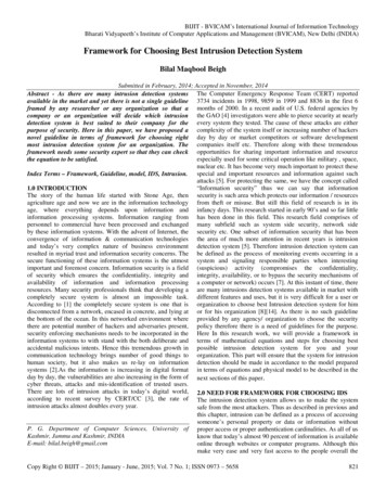
Towards Real-Time Intrusion Detectionfor NetFlow and IPFIXRick Hofstede , Václav Bartoš† , Anna Sperotto , Aiko Pras Design and Analysis of Communication Systems (DACS), Centre for Telematics and Information Technology (CTIT)University of Twente, Enschede, The Netherlands{r.j.hofstede, a.sperotto, a.pras}@utwente.nl† IT4Innovations Centre of ExcellenceBrno University of Technology, Brno, Czech Republicibartosv@fit.vutbr.czAbstract—DDoS attacks bring serious economic and technicaldamage to networks and enterprises. Timely detection andmitigation are therefore of great importance. However, when flowmonitoring systems are used for intrusion detection, as it is oftenthe case in campus, enterprise and backbone networks, timelydata analysis is constrained by the architecture of NetFlow andIPFIX. In their current architecture, the analysis is performedafter certain timeouts, which generally delays the intrusiondetection for several minutes. This paper presents a functionalextension for both NetFlow and IPFIX flow exporters, to allowfor timely intrusion detection and mitigation of large floodingattacks. The contribution of this paper is threefold. First, weintegrate a lightweight intrusion detection module into a flowexporter, which moves detection closer to the traffic observationpoint. Second, our approach mitigates attacks in near real-timeby instructing firewalls to filter malicious traffic. Third, we filterflow data of malicious traffic to prevent flow collectors fromoverload. We validate our approach by means of a prototypethat has been deployed on a backbone link of the Czech nationalresearch and education network CESNET.Index Terms—Internet measurements, Denial of service, Intrusion detection, NetFlow, IPFIX, Flow monitoring.I. I NTRODUCTIONMassive DDoS attacks are starting to become a new typeof warfare, in which networks and servers are overwhelmedby network traffic. For example, the Spamhaus Project [1] hasbeen targeted by attacks of more than 300 Gbps of bandwidthin early 2013 [2], large enough to overload Internet exchanges[3]. Other large flooding attacks that gained media attentionwere targeted at U.S. financial institutions in late 2012, wherecompromised Web servers were used as bots for creating amixture of high-volume TCP, UDP, ICMP and other IP-basedtraffic [4]. All these DDoS attacks are usually volume-based,and therefore suitable for detection in a flow-based manner.Flow export technologies, such as NetFlow [5] and IPFIX[6], provide a means for monitoring high-speed networks ina passive and scalable manner by aggregating packets intoflows. Flows are defined in [7] as sets of IP packets passingan observation point in the network during a certain timeinterval, such that all packets belonging to a particular flowhave a set of common properties. A typical deployment offlow export technologies is shown in Fig. 1. Flow exportersISBN 978-3-901882-53-1, 9th CNSM and Workshops 2013 IFIPAnalysis:IDSFlowCollector21Flow ExporterInternetForwardingDeviceFirewallLANFig. 1: Typical flow monitoring system deployment.receive raw packets and aggregate them into flows, whichis commonly referred to as flow metering. They can be partof forwarding devices (e.g. switches and routers), or separatedevices that are dedicated to the task of flow export, as shownin Fig. 1. After a flow is considered to have terminated,flow data is exported to flow collectors for storage and preprocessing. Finally, analysis applications, such as intrusiondetection systems (IDSs), retrieve flow data and analyze it [8]–[10], and potentially send out alerts or instruct firewalls.Due to the design of NetFlow and IPFIX, flow-based IDSsare subject to delays during flow metering and collection [11].These delays are in particular a consequence of timeouts forexpiring flow records as part of the flow metering process, andprocessing times of flow collectors. Considering the defaultidle timeout applied by several vendors and the processingtimes of state-of-the-art flow collectors, this usually results inIDS detection delays in the order of minutes. Nevertheless, itis important to detect and mitigate as early as possible to limitthe potential damage brought by large attacks, such as deviceoverload and link capacity exhaustion. Our intuition tells usthat moving parts of the detection process closer to the sourcemay reduce detection times drastically. Given that a timelydetection allows for timely mitigation, we propose a functional227
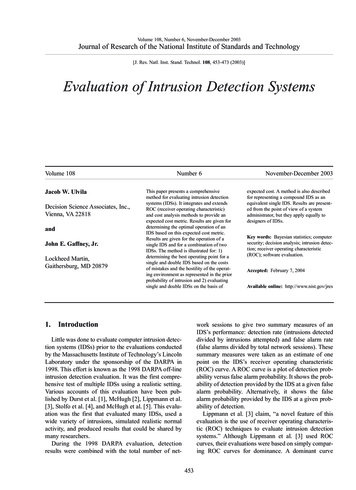
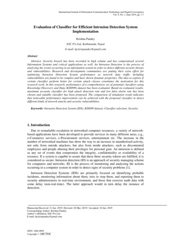
50(1)4010(4)(3)5000:0030PPF15BPF (k)Flow records / s (k)2020(2)1006:0012:0018:00(a) Flow record creations00:00000:0006:0012:0018:0000:00(b) Bytes per flow (BPF)70605040302010000:0006:0012:0018:0000:00(c) Packets per flow (PPF)Fig. 2: Flow-Based DDoS Attack Metrics.extension for flow exporters that integrates intrusion detectioninto the flow metering process. This avoids the delays incurredin typical flow monitoring systems and has the followingadvantages:1) Mitigation of DDoS flooding attacks by blocking malicious traffic before it reaches the LAN (as illustrated by(1) in Fig. 1).2) Mitigation of DDoS flooding attacks by filtering malicious flow data before it reaches and potentially overloads a flow collector (as illustrated by (2) in Fig. 1). Weknow from our operational experience that DDoS attacksoften cause flow data loss due to collector overload[12]. Moreover, European backbone operators have alsoconfirmed this problem in discussions we had with them.Typical values for the idle timeout applied for expiringflow records range from 15 seconds (default value appliedin Cisco’s IOS [13]) to 60 seconds (default value appliedin Juniper’s Junos [14]). In addition, flow collectors oftenwork based on time slots, which causes flow data to becomeavailable to analysis application only after the next time slothas started. For example, the state-of-the-art flow collectorNfSen uses time slots of 5 minutes, resulting in an averagedelay of 150 seconds (2.5 minutes). The average delay betweenthe moment in which a packet is metered and the time atwhich flow data is made available to analysis applications, istherefore at least 165 seconds, considering an idle timeout of15 seconds. In this paper, we analyze whether our approachcan reduce the delay up to 10% of this value. Besides thisrequirement, we target an intrusion detection module thatis lightweight, having a minimal performance footprint of10% in terms of CPU usage and memory consumption ona flow exporter. This is important since exporter operation isconsidered time-critical. Last, the accuracy of our intrusiondetection module should be high enough, to ascertain a lownumber of false positives/negatives.This paper is structured as follows. We start by analyzingflow-level characteristics of flooding attacks, mainly considering metrics that can be monitored in a lightweight manner(i.e. with a minimal performance footprint) on a flow exporter.Based on these findings, which are presented in Section II, westudy existing flooding attack detection algorithms that canbe modified to support the previously found metrics. Thesealgorithms are presented in Section III. In Section IV, weISBN 978-3-901882-53-1, 9th CNSM and Workshops 2013 IFIPpresent both the prototype that is used to validate whetherall identified requirements have been fulfilled, and the utilizeddatasets. Validation results are presented in Section V, togetherwith an example of the prototype in operation on a backbonelink. The feasibility of this work in terms of deployabilityon various high-end forwarding platforms is discussed inSection VI. Finally, we draw our conclusions in Section VII.II. DD O S ATTACK M ETRICSFlooding attacks are a type of (D)DoS attack that aim atexhausting targets’ resources by overloading them with largeamounts of traffic or (incomplete) connection attempts. Asevery connection attempt uses a different source port numberand therefore results in a new flow, large numbers of flowrecords are exported to flow collectors, effectively cancelingout the data aggregation advantage provided by flow exporttechnologies. In case a target replies to a connection attempt,two flow records are exported per attempt. The same characteristics may apply to (large) network scans. Flow collectorsneed to process all resulting records, consisting of only a fewpackets and bytes, which may be more than they can handle.In this section, we analyze which flow-level traffic metricsare suitable for lightweight detection of attacks on a flowexporter. Sadre et al. have previously identified four trafficmetrics that change significantly during a DDoS floodingattack: flow record creations per second, average flow duration,average number of bytes per flow, and average number ofpackets per flow [12]. All but the average flow duration can bemonitored on a flow exporter by using only counters, withoutthe need to access and process each individual flow record afterexpiration. This makes these metrics particularly interestingfor this work, in which we aim at designing a lightweightintrusion detection module for detecting large flooding attacks.Time-series of the three considered metrics are shown inFig. 2. The subfigures show data from one of the backbonelinks of the Czech national research and education networkCESNET in November 2012. The number of flow recordcreations per second is shown in Fig. 2a. The diurnal pattern isclearly identifiable and several peaks can be observed. Giventhe flow-level characteristics of flooding attacks, we assumethe peaks labeled with a number to indicate the presence ofsuch attacks. We have validated this assumption by manuallyverifying the presence of scanning and flooding attacks in theflow data.228
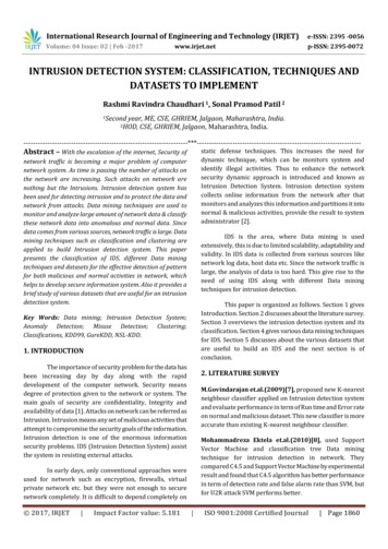
footprint justifies the use of Algorithm 2 in terms of accuracy,will be investigated later in this paper.Both algorithms rely on EWMA for calculating the meanover past values, which we use for forecasting the next value.Previous works have shown that EWMA can be used foranomaly detection (e.g. [15], [16]). It is defined as follows:Benign usTrafficSection 2Section 3Fig. 3: Detection Workflow.The number of bytes per flow (BPF) and packets per flow(PPF) are shown in Fig. 2b and Fig. 2c, respectively. Althoughthe attacks identified in Fig. 2a can be observed as negativepeaks here as well, the figures also show many other peaks,which make these metrics noisy. What can be confirmed fromthese figures, however, is that the attacks identified in Fig. 2aconsist of many small flows with few and small packets.Out of the three presented metrics in Fig. 2, the number offlow record creations (Fig. 2a) appears to be the most suitablemetric for our purposes for the following reasons. First, itshows the least amount of noise, peaks are clearly identifiable,and the identified peaks have been confirmed to be attacks, assubstantiated by the other metrics. Second, this metric is thebest to fulfill the requirement of being lightweight, as onlya single counter is needed that has to be reset after everymeasurement interval.Although we have shown only day-long time-series inFig. 2, we have verified that our conclusions are valid for thewhole dataset. We will therefore use the number of flow recordcreations for our traffic measurements, as shown in Fig. 3.These measurements are performed in a continuous fashionand used as input for a detection algorithm, which on its turnclassifies a measurement (sample) as benign or malicious. Twodetection algorithms are discussed in the next section.Algorithm 2: Algorithm 1, extended by seasonality modeling.Although the second algorithm may intuitively be considered more accurate, it is likely to have a larger performancefootprint in terms of memory consumption and processingcomplexity than the first algorithm, since more data needsto be stored and processed. Whether the larger performanceISBN 978-3-901882-53-1, 9th CNSM and Workshops 2013 IFIP α · xt (1 α) · x̄t 1(1) x̄t ,(2)where xt is the measured value, x̄t is the weighted mean overcurrent and past values at time t, x̂t 1 the value forecasted fortime t 1, and α (0, 1) a parameter which determines therate in which previous values are discarded. When the valueof xt becomes known, both the forecasting error et and anupper threshold Tupper,t can be calculated:et xt x̂t(3)Tupper,t x̂t max(cthreshold · σe,t , Mmin ) ,(4)where cthreshold is a constant and σe,t the standard deviationof previous forecasting errors. Mmin is a margin that isadded to the measurement x̂t to avoid instability in casecthreshold · σe,t is small. This solution prevents small peaksduring quiet periods to be considered anomalous. Note that wedo only consider an upper threshold and no lower threshold,since flooding attacks result, by definition, in a greater inputvalue in terms of flow record creations than the forecastedvalue (as discussed in Section II).Reporting an anomaly every time the upper thresholdhas been exceeded might cause a large number of falsepositives. To overcome this problem, we use a cumulativesum (CUSUM), which is widely used in anomaly detectionalgorithms [15], [17], [18]. The differences between the measurement and the upper threshold are summed (St ), and ananomaly is detected when the sum exceeds threshold Tcusum,t :III. D ETECTION A LGORITHMSIn this paper we consider an anomaly-based intrusion detection approach. One method for performing anomaly detectionbased on the analysis of time-series is forecasting, whichuses previous measurements for forecasting the next value.If the measured value does not lie within a certain rangeof the forecasted value, a measurement sample is consideredmalicious and an anomaly has been detected. In this paper, weconsider the following two algorithms:Algorithm 1: Exponentially weighted moving average(EWMA) for mean calculation, extended by thresholdsand a cumulative sum (CUSUM) [15]. We consider thisour basic algorithm.x̄tx̂t 1St max(St 1 (xt Tupper,t ), 0)(5)Tcusum,t ccusum · σe,t ,(6)where ccusum is a constant. A measurement is flagged anomalous every time Tcusum,t has been exceeded. To improve theprecision of anomaly end time detection, we use an upperbound on St to let St decrease faster after xt has decreased.The presented algorithm relies only on the forecasted valueand the measured value. Due to the daily periodicity ofnetwork traffic and the quick rises and falls of network utilization during mornings and evenings, respectively, the detectionalgorithm may benefit from a longer history. Our secondconsidered detection algorithm uses the Holt-Winters Additiveforecasting method for modeling seasonal components [19]:By adding a linear and a seasonal component to a base signal,the next value is forecasted. As a consequence of the dailyperiodicity of network traffic, we use day-long seasons. Sincewe do not identify a significant linear trend in network trafficat this timescale, we disregard the linear component. Theweighted mean (EWMA) of the base component is calculatedbased on previous measurements on the same day, while the229
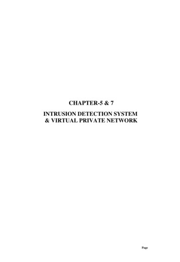
Processing pluginFilter rithmBlacklistFirewallConsoleFig. 4: Prototype Architecture.mean of the seasonal component is calculated over valuesat the same time in previous days. We define these twocomponents as follows:α · (xt st m ) (1 α) · bt 1bt st γ · (xt bt ) (1 γ) · st m(8) bt st ,(9)x̂t 1(7)where bt and st are the base and seasonal componentsof the forecasted value x̂t 1 , respectively, m is the seasonlength (i.e. number of measurement intervals per day, sincenetwork traffic shows daily periodicity), and γ (0, 1) aparameter which determines the rate in which previous valuesare discarded. The previous values in this case are not fromthe previous measurement interval, but from the same intervalin the previous season (i.e. day). The initial base value is setto the average of all measurement values in the first season.Therefore, a training period of one season is needed.The use of day-long seasons and small measurement intervals results in a large number of measurement values perseason. To support our requirement of being lightweight,we only store seasonal values every hour and interpolatebetween those. This also reduces measurement noise, whichwould otherwise imprint in the seasonal values. Besides that,precautions need to be taken to not let measurements duringanomalies influence the forecasts, which can be accomplishedby not updating st , bt and et during an anomaly. This is because we aim at forecasting non-anomalous network behavior.Another improvement made to the algorithm is to separatealgorithm states for weekdays and weekends, since the trafficbehavior usually varies significantly between these types ofdays. As such, forecasting of weekend days is done basedon the traffic behavior of the previous weekend, instead ofworking days. Analogously for weekdays.Siris et al. have shown that an interval between 5 and20 seconds yields best results for detecting flooding attacksusing the CUSUM method [15]. Our measurements haveshown that an interval of 5 seconds indeed results in themost accurate detection results, but an extensive comparisonof various interval lengths is out of the scope of this paper.A. PrototypeOur prototype implements both the traffic measurementsbased on the metric chosen in Section II (i.e. number of flowrecords creations) and the detection algorithms presented inSection III. It has been developed as a plugin for INVEATECH’s FlowMon platform, which has been selected bothbecause we have full control over it in our networks, andbecause of its highly customizable architecture based onplugins for data input, flow record processing, filtering, andexport. The prototype has been designed as a hybrid processingand filtering plugin. Default input and export plugins fromINVEA-TECH are used for packet capturing and NetFlow andIPFIX data export. Information gathered by the prototype, suchas detected anomalies, are sent to a console. The completearchitecture is depicted in Fig. 4.The intrusion detection module has been implemented asa processing plugin. After every measurement interval, thealgorithm is run and the measurement sample is classifiedas benign or malicious. This result is then passed on to afilter plugin, which is used for attack mitigation. When measurement samples are classified as benign, the correspondingflow records are passed on to the export plugin. Otherwise,the filter plugin identifies attackers as soon as an attack hasbeen detected. Attackers are identified by counting the numberof exported flow records per source IP address. When morethan F flow records per second with less than 3 packets andidentical source IP address have been exported, the address isadded to a blacklist. Measurements have shown that F 200is high enough to ascertain that a blacklisted host was floodinga network or host, and that benign hosts should never becomeblacklisted. In the case of attacks with spoofed IP addresses,one could also consider blacklisting destination addresses. Wehave measured the effects of this approach as well, but sourceaddress blacklisting has yielded slightly better results.After identification of the attackers, the filter plugin performs two actions, which correspond to the contributionsidentified in Section I:1) Firewall rules are composed and sent to a firewall toblock the attackers’ traffic. This corresponds to (1) inFig. 1.2) Flow records with the attackers’ IP addresses are filteredto reduce the stream of flow records sent to the collector.This corresponds to (2) in Fig. 1.IV. VALIDATION S ETUPThis section describes the setup used for validating ourwork. We start by discussing the developed prototype inSection IV-A, after which we provide details on the twodatasets used for validating our requirements in Section IV-B.ISBN 978-3-901882-53-1, 9th CNSM and Workshops 2013 IFIPWhen an anomaly has ended, the composed rule is removedfrom the firewall, counting of exported flow records is stopped,230
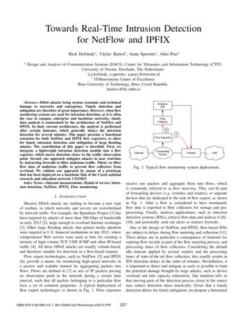
1Detection Rate (DR)Detection Rate (DR)10.90.8span 900span 1200span 1800span 36000.70.600.10.20.30.40.5False Positive Rate (FPR) - ccusum 50.90.8span 900span 1200span 1800span 36000.70.60.600.10.20.30.40.5False Positive Rate (FPR) - ccusum 70.6Fig. 5: Receiver Operating Characteristics (ROC) for Algorithm 1.TABLE I: DatasetsDurationA. AccuracyDataset 1Dataset 214 days10 daysPeriodAugust/September 2012October/November 2012Flows10.0 G (717.0 M per day)6.7 G (668.9 M per day)Packets257.1 G (18.4 G per day)186.7 G (18.7 G per day)Bytes134.5 T (9.6 T per day)128.5 T (12.8 T per aximum:5s5m, 55s2h, 41m, 50sMinimum:Average:Maximum:The accuracy of both detection algorithms is visualized bythe Receiver Operating Characteristics (ROC) curves shownin Fig. 5 and 6. The curves show the impact of the constantcthreshold on the Detection Rate (DR) and the False Positive Rate (FPR). The DR is a measure for the number ofattacks that have been detected correctly and is defined asfollows [20]:5s15m, 55s2h, 48m, 55sand all counters are reset. The filtering of flow records isstopped after Tidle seconds, where Tidle is the idle timeoutof the flow exporter, to make sure that flow records in theexporter’s flow cache that still belong to the attack are filtered.B. DatasetThe dataset used for validating the detection algorithms hasbeen captured on a backbone link of the CESNET networkin August/September 2012. This link has a wire-speed of 10Gbps with an average throughput of 3 Gbps during workinghours. The dataset comprises 14 days of measurements, composed of the number of flow record creations, packets andbytes per measurement interval (details are listed in Table I,Dataset 1). To establish a ground truth for validation, wehave manually identified anomalies that show a high intensityin the number of flow records. Samples belonging to ananomalous interval are labeled malicious. Other samples arelabeled benign.V. VALIDATION R ESULTSIn this section we validate whether our approach meets therequirements identified in Section I. We start by validating theaccuracy in Section V-A, mainly because of the fact that anintrusion detection module with a poor accuracy would be useless in any setup. After choosing the algorithm that performsbest in terms of accuracy, we validate the response time andperformance footprint of this algorithm in Section V-B andSection V-C, respectively.ISBN 978-3-901882-53-1, 9th CNSM and Workshops 2013 IFIPDR #{detected attacks}#{attacks}(10)The total number of attacks is determined by consideringconsecutive malicious samples to belong to the same attack.An anomaly is considered detected if approximately 50% ofthe samples is flagged malicious. The FPR is the ratio betweenthe number of samples incorrectly flagged malicious and thenumber of samples labeled benign. In contrast to the morecommon practice of plotting the True Positive Rate (TPR, ratiobetween the number of samples correctly flagged maliciousand the number of samples labeled malicious) versus the FPR,we plot the DR versus the FPR. This is because we do notrequire our algorithm to flag all samples of an anomaly, aslong as the ones with a high intensity are catched. Each curvein the plots shows the accuracy for a different combination ofspan and ccusum . Span represents the length in seconds of thehistory considered by the detection algorithm. As the algorithmis only aware of the number of measurement intervals and notof durations, we convert this time window to measurementintervals by dividing it by the length of a measurement interval.As such, it is used for calculating α (α N2 1 , where N isthe number of intervals [16]) and for determining the numberof values considered in calculating the standard deviation offorecasting errors σe,t . Besides span and ccusum , all otherparameters have been fixed: Mmin 7000 (Algorithm 1and 2), γ 0.4 (Algorithm 2).Several observations can be made regarding the performanceof Algorithm 1 in Fig. 5. First, it is clear that the differencein ccusum has little impact on the DR and FPR. Each pairof curves with the same span shows very similar growth.Second, increasing the span has little impact on the DR aswell, but it increases the FPR significantly. This is because231
1Detection Rate (DR)Detection Rate (DR)10.90.8span 1800span 3600span 5400span 72000.70.600.00050.001False Positive Rate (FPR) - ccusum 50.90.8span 1800span 3600span 5400span 72000.70.60.001500.00050.001False Positive Rate (FPR) - ccusum 70.0015Fig. 6: Receiver Operating Characteristics (ROC) for Algorithm 2.4010.83025CDFResponse time (s)35200.60.4150.2105000.511.5Relative attack intensity22.50(a) Response times for various attack intensities.510152025Response time (s)303540(b) CDF of the response time.Fig. 7: Response Times of Algorithm 2.the forecast adapts slower to network traffic changes, such asdiurnal patterns, and small deviations in the measurements are(incorrectly) flagged as malicious. Third, increasing cthresholdaffects the DR negatively: The highest DRs in the figureare achieved when the lowest cthreshold is used. This isbecause the resulting higher upper threshold Tupper,t willcause certain anomalies to stay below the threshold, resultingin a higher number of FNs. In the case of Fig. 5, cthreshold {1.5, 2, 3, 5}. In our experiments, a span of 900 seconds anda cthreshold of 3 yield the most optimal combination of a highDR (92%), while maintaining a low FPR (6%). In a typicaldeployment scenario as shown in Fig. 1, however, this FPR isunacceptable as benign hosts may be blocked erroneously byour approach.The ROC curve for various combinations of parametervalues for Algorithm 2 is shown in Fig. 6. Similar parametervalues as for Algorithm 1 yield similar DRs, while the FPRis significantly lower, namely between 0% and 0.01%. Highervalues of cthreshold yield lower DRs, for the same reason asdescribed for Algorithm 1. Again, cthreshold {1.5, 2, 3, 5}.When a span 3600 seconds is used, the FPR increasesslightly for small values of cthreshold , although still being verysmall (0.1%).In general, we conclude that Algorithm 2 is more suitableas a detection algorithm in our situation than Algorithm 1,since the FPRs are much lower while similar (high) DRs areISBN 978-3-901882-53-1, 9th CNSM and Workshops 2013 IFIPmaintained. We therefore conclude that the higher accuracyof this algorithm should excuse the additional performancefootprint on the flow exporter. In the remainder of this section,we will therefore only consider Algorithm 2.B. Response TimeThe main goal of this paper is to perform flow-basedintrusion detection in near real-time. An important metric inthe validation is therefore the response time. We define theresponse time as the time between the moment in whichthe algorithm detects an anomaly and the beginning of theanomaly. A scatter plot showing response times for variousattack intensities is shown in Fig. 7a, where we define therelative attack intensity as the fraction between the forecastingerror (see (3)) and the forecasted number of flow records:et(11)x̂t 1The response time is always a multiple of 5 seconds, as thisis the length of our measurement intervals. A response timeof 5 seconds means that an anomaly has been detected withinthe same sample as the anomaly has started. As shown inthe figure, most anomalies with a relative intensity larger than0.3 are detected within 10 seconds. Outliers are the result ofattacks that do not reach their full intensity right from the start.Anomalies with a relative intensity 0.3 are mostly detectedwithin 40 seconds. However, these anomalies are not the main232
800Flow records / 5s )04:0008:0012:0016:0020:0000:0004:0008:0012:00Fig. 8: Prototype Mitigation Results.target of our work as their potential damage to networks andhosts will be limited. Another view on the response times ofthe algorithm is shown in Fig. 7b, where the CDF is plottedfor each potential response time. It can be observed that 68%of all anomalies is detected within 5 seconds and 90% of theanomalies within 15 seconds. Note that these response timesare even lower than typical idle timeouts of flow exporters, asshown in Section I.An example of the prototype in operation is shown in Fig. 8.The figure shows the number of flow record creations, asmeasured by the processing plugin per measurement intervalof 5 seconds, and the number of flow records dropped by thefilter plugin per measurement interval, over a period of 36hours. This measurement period is a subset of Dataset 2 (seeTable I). Several large anomalies can be identified, labeled as(1)-(6). The anomalies (1), (5) and (6) are clearly smallerthan the others and are dropped largely or completely by thefilter plugin. However, the main focus of our work is on verylarge anomalies, such as the anomalies marked as (2), (3) and(4). Anomaly (2) consists of 755k flow records per 5 seconds,while roughly 40k flow records have been forecasted. Out ofthese 755k flow records, our prototype is able to mitigate 715k.Anomaly (3) and (4) are both part of one longer anomaly,which is dropped partly throughout the duration of the attack.Anomaly (3) is mitigated completely, as the number of passedflow records roughly equals the forecasted number of flowrecords for measurement intervals during the attack (23k).Anomaly (4) is mitigated partially, where about 50% of thetotal number of flow records is dropped. When anomalies havenot been dropped completely, one or more attackers generatedless flows than the threshold of F 200 per second. Wedo not consider this problematic since the number of passedflow records (40k per measurement interval) is in principlenot causing collector overload, as this number equals thenumber of benign flow records at midday. Anomalies outsidethe visualized part of Datas
for NetFlow and IPFIX Rick Hofstede , Vaclav Barto sˇy, Anna Sperotto , Aiko Pras Design and Analysis of Communication Systems (DACS), Centre for Telematics and Information Technology (CTIT) University of Twente, Enschede, The Netherlands fr.j.hofstede, a.sperotto, a.prasg@utwente.nl yIT4Innovations Centre of Excellence