Transcription
Real-Time Scheduling with Regenerative Energy1C. Moser 1 , D. Brunelli 2 , L. Thiele 1 and L. Benini 2Swiss Federal Institute of Technology (ETH) Zurich, Switzerland{moser thiele}@tik.ee.ethz.ch2University of Bologna, Italy{dbrunelli lbenini}@deis.unibo.itAbstractThis paper investigates real-time scheduling in a systemwhose energy reservoir is replenished by an environmentalpower source. The execution of tasks is deemed primarilyenergy-driven, i.e., a task may only respect its deadline ifits energy demand can be satisfied early enough. Hence,a useful scheduling policy should account for properties ofthe energy source, capacity of the energy storage as well aspower dissipation of the single tasks. We show that conventional scheduling algorithms (like e.g. EDF) are not suitable for this scenario. Based on this motivation, we stateand prove optimal scheduling algorithms that jointly handle constraints from both energy and time domain. Furthermore, an offline schedulability test for a set of periodicor even bursty tasks is presented. Finally, we validate theproposed theory by means of simulation and compare ouralgorithms with the classical Earliest Deadline First Algorithm.real-time responsiveness of these inherently energy constrained devices can be guaranteed. Is it possible to schedule a given set of tasks within their deadlines and – ifyes – which scheduling policy guarantees schedulability?– Clearly, the answers to this questions depend on parameters like the capacity of the battery and the impinging lightintensity. Unfortunately, the latter is highly unstable andcomplicates the search for online scheduling algorithms aswell as admittance tests.The Earliest Deadline First (EDF) algorithm has beenproven to be optimum with respect to the schedulability of agiven taskset in traditional time-driven scheduling. The following example shows why greedy scheduling algorithms(like EDF) are not suitable in the context of this paper.storedenergytimetaskexecution12time1. IntroductionOne of the key challenges of wireless sensor networksis the energy supply of the single nodes. As for manyother battery-operated embedded systems, a sensor’s lifetime, size and cost can be significantly improved by appropriate energy management. In particular, sensor nodes aredeployed at places where manual recharging or replacementof batteries is not practical. In order for sensor networks tobecome a ubiquitous part of our environment, alternativepower sources must be employed. Therefore, environmental energy harvesting is deemed a promising approach.In [6], several technologies have been discussed how,e.g., solar, thermal, kinetic or vibrational energy may beextracted from a node’s physical environment. Several prototypes like Heliomote [5] or Prometheus [3] could demonstrate that solar energy is a viable power source to achieveperpetual operation. However, it remains unclear howProceedings of the 18th Euromicro Conference on Real-Time Systems (ECRTS’06)0-7695-2619-5 /06 20.00 2006IEEEstoredenergytimetaskexecution21timeFigure 1. Greedy vs. lazy schedulingLet us consider a node with an energy harvesting unitthat replenishes a battery with constant power. Now, thisnode has to perform an arriving task ”1” that has to be finished until a certain deadline. Meanwhile, a second task ”2”has to be executed within a shorter time interval that is againgiven by an arrival time and a deadline. In Figure 1, the arrival times and deadlines of these tasks are indicated by upand down arrows respectively. As depicted in the top diagrams, a greedy scheduling strategy violates the deadline
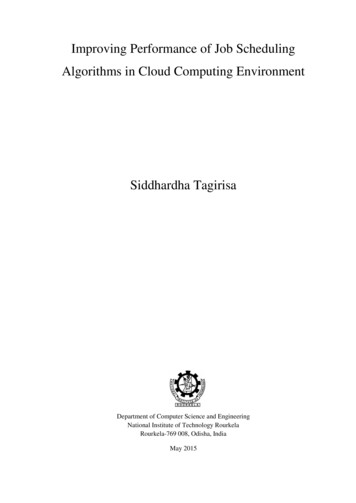
of task ”2” since it dispenses overhasty the stored energyby driving task ”1”. When the energy is required to execute the second task, the battery level is not sufficient tomeet the deadline. In this example, however, a schedulingstrategy that hesitates to spend energy on task ”1” meetsboth deadlines. The bottom plots illustrate how the LazyScheduling paradigm described in this paper outperforms anaive, greedy approach like EDF in the described situation.The research presented in this paper is directed towardssensor nodes. But in general, our results apply for allkind of energy harvesting systems which must scheduleprocesses under deadline constraints: We claim, that ourscheduling algorithms are not only energy-aware, but trulyenergy-driven. This insight originates from the fact, thatenergy – contrary to the computation resource ”time” – isstorable. As a consequence, every time we withdraw energy from the battery to execute a task, we change the stateof our scheduling system. That is, after having scheduled afirst task the next task will encounter a lower energy level inthe system which in turn will affect its own execution. Thisis not the case in conventional real-time scheduling wheretime just elapses either used or unused.The following new results are described in this paper: We present an energy-driven scheduling scenario for asystem whose energy storage is recharged by an environmental source. For this scenario, we state and prove optimal onlinealgorithms that dynamically assign energy to arrivingtasks. These algorithms are energy-clairvoyant, i.e.,scheduling decisions are driven by the future incomingenergy. We present an admittance test that decides, whethera set of tasks can be scheduled with the energy produced by the harvesting unit. For this purpose, weintroduce the concept of energy variability characterization curves (EVCC). Finally, we propose practical algorithms which predictthe future harvested energy with the help of EVCCs.Simulation results demonstrate the benefits of our algorithms compared to the classical Earliest DeadlineFirst Algorithm.The remainder of the paper is organized as follows: Inthe next section, we discuss how our approach differs fromrelated work. Subsequently, Section 3 gives definitions thatare essential for the understanding of the paper. In Section 4, we present Lazy Scheduling Algorithms for optimalonline scheduling. Admittance tests for arbitrary tasksetsare the topic of Section 5. Simulation Results are presentedin Section 6 and Section 7 concludes the paper.Proceedings of the 18th Euromicro Conference on Real-Time Systems (ECRTS’06)0-7695-2619-5 /06 20.00 2006IEEE2. Related workIn [4], the authors use a similar model of the powersource as we do. But instead of executing concrete tasks ina real-time fashion, they propose tuning a node’s duty cycledependent on the parameters of the power source. Nodesswitch between active and sleep mode and try to achievesustainable operation. This approach only indirectly addresses real-time responsiveness: It determines the latencyresulting from the sleep duration.The approach in [7] is restricted to a very special offlinescheduling problem: Periodic tasks with certain rewardsare scheduled within their deadlines according to a givenenergy budget. The overall goal is to maximize the sumof rewards. Therefore, energy savings are achieved usingDynamic Voltage Scaling (DVS). The energy source is assumed to be solar and comprises two simple states: day andnight. Hence the authors conclude that the capacity of thebattery must be at least equal to the cumulated energy ofthose tasks, that have to be executed at night. In contrast,our work deals with a much more detailed model of the energy source. We focus on scheduling decisions for the online case when the scheduler is indeed energy-constraint. Indoing so, we derive valuable bounds on the necessary battery size for arbitrary energy sources and tasksets.The research presented in [1] is dedicated to offline algorithms for scheduling a set of periodic tasks with a commondeadline. Within this so-called ”frames”, the order of taskexecution is not crucial for whether the taskset is schedulable or not. The power scavenged by the energy source isassumed to be constant. Again – by using DVS – the energyconsumption is minimized while still respecting deadlines.Contrary to this work, our systems (e.g. sensor nodes) arepredominantly energy constrained and the energy demandof the tasks is fixed (no DVS). We propose algorithms thatmake best use of the available energy. Provided that theaverage harvested power is sufficient for continuous operation, our algorithms minimize the necessary battery capacity.3. System model and assumptionsThe paper deals with a scheduling scenario depicted inFig. 2. At some time t, an energy source harvests ambient energy and converts it into electrical power PS (t). Thispower can be stored in a device with capacity C. The storedenergy is denoted as EC C. On the other hand, a computing device drains power PD (t) from the storage and uses itto process tasks with arrival time ai , energy demand ei anddeadline di . We assume that only one task is executed attime t and preemptions are allowed. The following subsections define the relations between these quantities in moredetail.
energy sourceSSPS(t)EC(t)CCenergy storagePD(t)J1J1a1, e1, d1J2JtΔiΔ Figure 3. Power trace and energy variabilitycharacterization curve (EVCC)2a2, e2, d23.1. Energy sourceMany environmental power sources are highly variablewith time. Hence, in many cases some charging circuitry isnecessary to optimize the charging process and increase thelifetime of the storage device. In our model, the power PSincorporates all losses caused by power conversion as wellas charging process. In other words, we denote PS (t) thecharging power that is actually fed into the energy storage. The respective energy ES in the time interval [t1 , t2 ] isgiven as t2PS (t)dt .ES (t1 , t2 ) t1In order to characterize the properties of an energy source,we define now energy variability characterization curves(EVCC) that bound the energy harvested in a certain interval Δ: The EVCCs l (Δ) and u (Δ)with Δ 0 bound therange of possible energy values ES as follows: l (t2 t1 ) ES (t1 , t2 ) u (t2 t1 ) t2 t1Given an energy source, e.g., a solar cell mounted in a building or outside, the EVCCs provide guarantees on the produced energy. For example, the lower curve denotes thatfor any time interval of length Δ, the produced energy is atleast l (Δ) (see Fig. 3). Two possible ways of deriving anEVCC for a given scenario are given below: A sliding window of length Δ is used to find the minimum/maximum energy produced by the energy sourcein any time interval [t1 , t2 ) with t2 t1 Δ. To thisend, one may use a long power trace or a set of tracesthat have been measured. Since the resulting EVCCbounds only the underlying traces, these traces mustbe selected carefully and have to be representative forthe assumed scenario. The energy source and its environment is formallymodeled and the resulting EVCC is computed.Proceedings of the 18th Euromicro Conference on Real-Time Systems (ECRTS’06)IEEEεl(Δi)ΔiFigure 2. Scheduling scenario0-7695-2619-5 /06 20.00 2006εl(Δi)DDcomputing devicetasksεl(Δ)PS(t)3.2. Energy storageWe assume an ideal energy storage (e.g. a battery) thatmay be charged up to its capacity C. According to thescheduling policy used, power PD (t) and the respective energy ED (t1 , t2 ) is drained from the storage to execute tasks.If no tasks are executed and the storage is consecutively replenished by the energy source, an energy overflow occurs.Consequently, we can derive the following relations:EC (t) CED (t1 , t2 ) EC (t1 ) ES (t1 , t2 ) t t2 t1EC (t2 ) EC (t1 ) ES (t1 , t2 ) ED (t1 , t2 ) t2 t13.3. Task schedulingAs illustrated in Fig. 2, we utilise the notion of a computing device that assigns energy EC from the storage todynamically arriving tasks. Here, we limit the power consumption PD (t) of the system to the maximum value Pmax .In other words, the processing device determines at anypoint in time how much power it uses, that is0 PD (t) Pmax .We assume tasks to be independent from each other andpreemptive. That is, the currently active task may be interrupted at any time and continued at a later time. If the nodedecides to assign power Pi (t) to the execution of task Jiduring the interval [t1 , t2 ], we denote the corresponding energy Ei (t1 , t2 ). The effective starting time si and finishingtime fi of task i are dependent on the scheduling strategyused: A task starting at time si will finish as soon as therequired amount of energy ei has been consumed by it. Wecan writefi min {t : Ei (si , t) ei } .We see that the actual running time (fi si ) of a task iis strongly dependent on the amount of power Pi (t) whichis driving the task during si t fi . In the best case,eiifa task may finish after the execution time wi Pmaxit is processed without interrupts and with the maximumpower Pmax .
4. Lazy Scheduling Algorithms LSAAfter having described our modeling assumptions, wewill now state and prove optimal scheduling algorithms. Insubsection 4.1 and 4.2, we will introduce two schedulingalgorithms that dynamically assign energy and time to arriving tasks. Theorems which prove optimality of both algorithms will follow in subsection 4.3.4.1. LSA-I for unlimited power PmaxWe start with a hypothetical system with infinitepower Pmax . As a result, a task’s execution time wicollapses to 0 if the available energy EC in the storage isequal to or greater than the task’s energy demand ei . Thisfact clearly simplifies the search for advantageous scheduling algorithms but at the same time contributes to the understanding of our problem. Furthermore, it should be mentioned that a theoretical node which runs a task in zero timecan be a good approximation for many practical scenarios.Whenever processing times wi are negligible compared tothe time to recharge the battery (i.e. Pmax PS (t)), theassumed model can be regarded as reasonable.For optimal task scheduling, the processing device has toselect between three power modes. The node may processtasks with the maximal power PD (t) Pmax or not atall (PD (t) 0). In between, the node may choose tospend only the currently incoming power PS (t) from theharvesting unit on tasks. Altogether, we consider a nodethat decides between PD (t) PS (t), PD (t) 0 andPD (t) to schedule arriving tasks.As already indicated in the introduction, the naive approach of simply scheduling tasks with the EDF algorithmmay result in unnecessary deadline violations (cp. Fig. 1).It may happen, that after the execution of task ”1” anothertask ”2” with an earlier deadline arrives. If now the requiredenergy is not available before the deadline of task ”2”, EDFscheduling produces a deadline violation. If task ”1” wouldwait instead of executing directly, this deadline violationmight have been avoidable. These considerations directlylead us to the principle of Lazy Scheduling: Gather environmental energy and process tasks only if it is necessary.The Lazy Scheduling Algorithm (LSA-I) for Pmax shown below attempts to assign energy to a set of tasksJi , i Q such that deadlines are respected. It is basedon the two following rules: Rule 1: If the current time t equals the deadline dj ofsome arrived but not yet finished task Jj , then finishits execution by draining energy (ej Ej (aj , t)) fromthe energy storage instantaneously, i.e. with PD (dj ) . Rule 2: We must not waste energy if we could spendProceedings of the 18th Euromicro Conference on Real-Time Systems (ECRTS’06)0-7695-2619-5 /06 20.00 2006IEEEit on task execution. Therefore, if we hit the capacitylimit (EC (t) C) at some times t, we execute the taskwith the earliest deadline using PD (t) PS (t). Rule 3: Rule 1 overrules Rule 2.Lazy Scheduling Algorithm LSA 1 (Pmax )Require: maintain a set of indices i Q of all ready butnot finished tasks JiPD (t) 0;while (true) dodj min{di : i Q};process task Jj with power PD (t);t current time;then add index k to Q;if t akthen remove index j from Q;if t fjthen EC (t) EC (t) ej Ej (aj , t);if t djremove index j from Q;PD (t) 0;if EC (t) C then PD (t) PS (t);The above algorithm is solely designed for schedulabletasksets and doesn’t account for possible deadline violations. If there is not enough energy available at the deadline of task (EC (dj ) ej Ej (aj , dj )) then the taskset isassumed to be not schedulable.Note that the LSA degenerates to an earliest deadlinefirst (EDF) policy, if C 0. On the other hand, we find anas late as possible (ALAP) policy for the case of C .4.2. LSA-II for limited power PmaxNow, we focus on how LSA-I must be adapted to handle limited power consumption and finite execution times.In doing so, we determine an optimal starting time s thatbalances the time and energy constraints for our schedulingscenario.The LSA-I algorithm instantaneously executes a task atits deadline. However, after the introduction of a finite, minei, LSA-II has to deterimal computation time wi Pmaxmine an earlier starting time in order to hold the respectivedeadline. The upper plots in Fig. 4 display a straightforwardALAP-translation of the starting time for task ”1”: To fulfillits time condition, task ”1” begins to execute at starting timee1. As illustrated, it may happen that shortlys1 d1 Pmaxafter s1 an unexpected task ”2” arrives. Assume that thisunexpected task ”2” is nested in task ”1”, i.e., it also hasan earlier deadline than ”1”. This scenario inevitably leadsto a deadline violation, although plenty of energy is available. This kind of timing conflict can be solved by shiftings1 to earlier times and thereby reserving time for the unpredictable task ”2” (see lower plots Fig. 4). But startingearlier, we risk to ”steal” energy that might be needed at
later times (compare Fig. 1). So – according to the ”lazy”principle – we have to take care that we don’t start too early.calculate the starting time s i ass i di storedenergytimetaskexecution1 2es1 d1- p1maxtimestoredenergyEC (ai ) ES (ai , di ).PmaxIf now the energy storage was filled before s i , starting execution at s i could yield EC (t) 0 at some time t di .Thus starting at s i means starting too early and one can finda better starting time s i by solving the following equationnumerically:ES (ai , s i ) C ES (ai , di ) (s i di )Pmax .timetaskexecution12times1Figure 4. ALAP vs. lazy schedulingFrom the above example, we learned that it may be disadvantageous to prearrange a starting time in such a way,that the stored energy EC cannot be used before the deadline of a task. If the processing device starts running attime s with Pmax and cannot consume all the available energy before the deadline d, time conflicts may occur. Onthe other hand, if we remember the introductory examplein Fig. 1, energy conflicts are possible if the stored energyEC (t) 0 at some time t d. Hence we can conclude thefollowing: The scheduler has to conserve the energy EC aslong as required, but must start processing the stored energy duly. Consequently, the optimal starting time s mustguarantee, that the processor could continuously use Pmaxin the interval [s, d] and empty the energy storage at time d.A necessary prerequisite for the calculation of the optimal starting time si is the knowledge of the incoming powerflow PS (t) for all future times t di . Finding useful predictions for the power PS (t) can be done, e.g., by analyzingtraces of the harvested power, as we will see in Section 6.In addition, we assume thatPS (t) Pmax t ,that is, the incoming power PS (t) from the harvesting unitnever exceeds the power consumption Pmax of a busy node.Besides from being a realistic model in many cases, thisassumption prevents us from dealing with possible energylosses.To calculate the optimal starting time si , we determinethe maximum amount of energy EC (ai ) ES (ai , di ) thatmay be processed by the node before di . Next, we compute the minimum time required to process this energy without interruption and shift this time interval of continuousprocessing just before the deadline di . In other words, weProceedings of the 18th Euromicro Conference on Real-Time Systems (ECRTS’06)0-7695-2619-5 /06 20.00 2006IEEEWe denote the optimal starting timesi max (s i , s i ).The pseudo-code of the Lazy Scheduling AlgorithmLSA-II is shown below. It is based on the following rules: Rule 1: EDF scheduling is used at time t for assigningthe processor to all waiting tasks with si t. Thecurrently running task is powered with PD (t) Pmax . Rule 2: If there is no waiting task i with si t andif EC (t) C, then all incoming power PS is used toprocess the task with the smallest deadline(PD (t) PS (t)). If there is no waiting task at all, the incomingpower is wasted.Lazy Scheduling Algorithm LSA 2 (Pmax const.)Require: maintain a set of indices i Q of all ready butnot finished tasks JiPD (t) 0;while (true) dodj min{di : i Q};calculate sj ;process task Jj with power PD (t);t current time;then add index k to Q;if t akthen remove index j from Q;if t fjif EC (t) C then PD (t) PS (t);then PD (t) Pmax ;if t sjThe calculation of si must be performed once the scheduler selects the task with the earliest deadline. If the scheduler is not energy-constraint, i.e., if the available energy ismore than the device can consume with power Pmax within[ai , di ], the starting time si will be before the current time t.Then, the resulting scheduling policy is EDF, which is reasonable, because only time constraints have to be satisfied.In summary, LSA-II can be classified as an energyclairvoyant adaptation of the Earliest Deadline First Algorithm. It changes its behaviour according to the amount of
available energy, the capacity C as well as the maximumpower consumption Pmax of the device. For example, thelower the power Pmax gets, the greedier LSA-II gets. Onthe other hand, high values of Pmax force LSA-II to hesitate and postpone the starting time s. For Pmax , allstarting times collapse to the respective deadlines, and weidentify LSA-I as a special case of LSA-II.4.3. Optimality proof for LSA I IIIn this section, we will show that the LSA-II algorithmis optimal in the following sense: If the algorithm can notschedule a given set of tasks no other algorithm is able todo so. Since LSA-I is just a special case of LSA-II, theconsiderations in this section are restricted to the case ofLSA-II.The scheduling scenario presented in this paper is inherently energy-driven. Hence, a scheduling algorithm yields adeadline violation if it fails to assign the energy ei to a taskbefore its deadline di . We distinguish between two types ofdeadline violations: A deadline cannot be respected since the timeis not sufficient to execute available energy withpower Pmax . At the deadline, unprocessed energy remains in the storage and we have EC (d) 0. We callthis the time limited case. A deadline violation occurs because the required energy is simply not available at the deadline. At thedeadline, the battery is exhausted (i.e., EC (d) 0).We denote the latter case energy limited.For the following theorems to hold we suppose that atinitialization of the system, we have a full capacity, i.e.,EC (ti ) C. Furthermore, we call the computing deviceidle if no task i is running with si t.Theorem 1 Let us suppose that the LSA-II algorithmschedules a set of tasks. At time d the deadline of a taskJ with arrival time a is missed and EC (d) 0. Thenthere exists a time t1 such that the sum of execution times ei(i) wi (i) Pmax of tasks with arrival and deadlinewithin time interval [t1 , d] exceeds d t1 .Proof 1 Let us suppose that t0 is the maximal time t0 dwhere the processor was idle. Clearly, such a time exists.We now show, that at t0 there is no task i with deadlinedi d waiting. At first, note that the processor is constantly operating on tasks in time interval (t0 , d]. Supposenow that there are such tasks waiting and task i is actuallythe one with the earliest deadline di among those. Then,as EC (d) 0 and because of the construction of si , wewould have si t0 . Therefore, the processor would actually process task i at time t0 which is a contradiction to theidleness.Proceedings of the 18th Euromicro Conference on Real-Time Systems (ECRTS’06)0-7695-2619-5 /06 20.00 2006IEEEBecause of the same argument, all tasks i arriving aftert0 with di d will have si ai . Therefore, LSA-II willattempt to directly execute them using an EDF strategy.Now let us determine time t1 t0 which is the largesttime t1 d such that the processor continuously operateson tasks i with di d. As we have si ai for all of thesetasks and as the processor operates on tasks with smallerdeadlines first (EDF), it operates in [t1 , d] only on tasks withai t1 and di d. As there is a deadline violation at timed, we can conclude that (i) wi d t1 where the sumis taken over all tasks with arrival and deadline within timeinterval [t1 , d].Theorem 2 Let us suppose that the LSA-II algorithmschedules a set of tasks. At time d the deadline of a taskJ with arrival time a is missed and EC (d) 0. Then thereexists a time t1 such that the sum of task energies (i) ei oftasks with arrival and deadline within time interval [t1 , d]exceeds C ES (t1 , d).Proof 2 Let time t1 d be the largest time such that (a)EC (t1 ) C and (b) there is no task i waiting with di d.Such a time exists as one could at least use the initializationtime ti with EC (ti ) C. As t1 is the last time instancewith the above properties, we can conclude that everywherein time interval [t1 , d] we either have (a) EC (t) C andthere is some task i waiting with di d or we have (b) andEC (t) C.It will now be shown that in both cases a) and b), energyis not used to advance any task j with dj d in time interval [t1 , d]. Note also, that all arriving energy ES (t1 , d) isused to advance tasks.In case a), all non-storable energy (i.e. all energy thatarrives from the source) is used to advance a waiting task,i.e., the one with the earliest deadline di d. In case b),the processor would operate on task J with dj d if thereis some time t2 [t1 , d] where there is no other task i withdi d waiting and sj t2 . But sj is calculated such thatthe processor could continuously work until dj . As dj dand EC (d) 0 this can not happen and sj t2 . Therefore,also in case b) energy is not used to advance any task j withdj d.As there is a deadline violation at time d, we can conclude that (i) ei C EC (t1 , d) where the sum is takenover all tasks with arrival and deadline within time interval[t1 , d].From the above two theorems we draw the followingconclusions: First, in the time limited case, there exists atime interval before the violated deadline with a larger accumulated computing time request than available time. Andsecond, in the energy limited case, there exists a time interval before the violated deadline with a larger accumulatedenergy request than what can be provided at best. Therefore, we conclude the following:
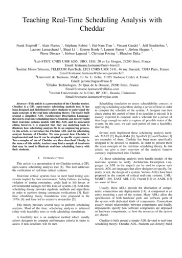
Corollary 1 (Optimality of Lazy Scheduling) If LSA-IIcannot schedule a given taskset, then no other schedulingalgorithm can. This holds even if the other algorithm knowsthe complete taskset in advance.If we can guarantee that there is no time interval with alarger accumulated computing time request than availabletime and no time interval with a larger accumulated energyrequest than what can be provided at best, then the tasksetis schedulable. This property will be used to determine theadmittance test described next.α1 (Δ)α1(Δ)482142126 Δ4p1 21246 Δp1 2, d1 1.5, e1 2Α(Δ)85. Admittance testIn this section, we will determine an offline schedulability test in case of periodic, sporadic or even bursty tasksets.In particular, given an energy source with lower EVCC l (Δ), an energy storage with capacity C and a set of periodic tasks Ji , i I with period pi , relative deadline diand energy demand ei , we would like to determine whetherall deadlines can be respected.To this end, let us first define for each task its arrivalcurve α(Δ) which denotes the maximal number of task arrivals in any time interval of length Δ. The notion of arrival curves to describe the arrival patterns of tasksets iswell known and has been used explicitly or implicitly in,e.g., [2], or [8]. To simplify the discussion, we limit ourselves to periodic tasks, but the whole formulation allowsto deal with much more general classes (sporadic or bursty)as well.In case of a periodic taskset, we have for periodic task Ji ,see also Fig. 5: Δ Δ 0αi (Δ) piIn order to determine the maximal energy demand in anytime interval of length Δ, we need to maximize the accumulated energy of all tasks having their arrival and deadlinewithin an interval of length Δ. To this end, we need to shiftthe corresponding arrival curve by the relative deadline. Incase of a periodic task Ji , this simply leads to: ei · αi (Δ di ) Δ diαi (Δ) 00 Δ diIn case of several periodic tasks that arrive concurrently,the total demand curve A(Δ) can be determined by justadding the individual contributions of each periodic task,see Fig. 5: αi (Δ)A(Δ) i IUsing the above defined quantities, we can formulateone of the major results of the paper which determines theschedulability of an arbitrary taskset:Proceedings of the 18th Euromicro Conference on Real-Time Systems (ECRTS’06)0-7695-2619-5 /06 20.00 2006IEEE42Δ12 4 6 8p1 2, d1 1.5, e1 2p2 3, d2 4, e2 1Figure 5. Examples of an arrival curve, a demand curve and a total demand curve in caseof periodic tasks.Theorem 3 (Schedulability Test) A given set of tasks Ji ,i I with arrival curves αi (Δ), energy demand ei andrelative deadline di is schedulable under the energy-drivenmodel with initially stored energy C, if and only if the following condition holds Δ 0A(Δ) min l (Δ) C , Pmax · Δ Here, A(Δ) i I ei · αi (Δ di ) denotes the total energy demand of the taskset in any time interval of length Δ, l (Δ) the energy variability characterization curve of theenergy source, C the capacity of the energy storage
and prove optimal scheduling algorithms that jointly han-dle constraints from both energy and time domain. Fur-thermore, an offline schedulability test for a set of periodic or even bursty tasks is presented. Finally, we validate the proposed theory by means of simulation and compare our algorithms with the classical Earliest Deadline First .