Transcription
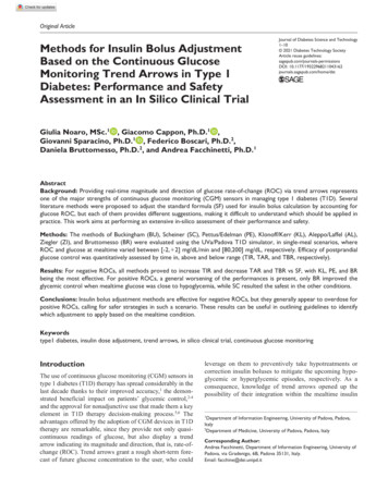
11043162Journal of Diabetes Science and TechnologyNoaro et alOriginal ArticleMethods for Insulin Bolus AdjustmentBased on the Continuous GlucoseMonitoring Trend Arrows in Type 1Diabetes: Performance and SafetyAssessment in an In Silico Clinical TrialJournal of Diabetes Science and Technology 1 –10 2021 Diabetes Technology SocietyArticle reuse /doi.org/10.1177/19322968211043162DOI: /dstGiulia Noaro, MSc.1 , Giacomo Cappon, Ph.D.1 ,Giovanni Sparacino, Ph.D.1 , Federico Boscari, Ph.D.2,Daniela Bruttomesso, Ph.D.2, and Andrea Facchinetti, Ph.D.1AbstractBackground: Providing real-time magnitude and direction of glucose rate-of-change (ROC) via trend arrows representsone of the major strengths of continuous glucose monitoring (CGM) sensors in managing type 1 diabetes (T1D). Severalliterature methods were proposed to adjust the standard formula (SF) used for insulin bolus calculation by accounting forglucose ROC, but each of them provides different suggestions, making it difficult to understand which should be applied inpractice. This work aims at performing an extensive in-silico assessment of their performance and safety.Methods: The methods of Buckingham (BU), Scheiner (SC), Pettus/Edelman (PE), Klonoff/Kerr (KL), Aleppo/Laffel (AL),Ziegler (ZI), and Bruttomesso (BR) were evaluated using the UVa/Padova T1D simulator, in single-meal scenarios, whereROC and glucose at mealtime varied between [-2, 2] mg/dL/min and [80,200] mg/dL, respectively. Efficacy of postprandialglucose control was quantitatively assessed by time in, above and below range (TIR, TAR, and TBR, respectively).Results: For negative ROCs, all methods proved to increase TIR and decrease TAR and TBR vs SF, with KL, PE, and BRbeing the most effective. For positive ROCs, a general worsening of the performances is present, only BR improved theglycemic control when mealtime glucose was close to hypoglycemia, while SC resulted the safest in the other conditions.Conclusions: Insulin bolus adjustment methods are effective for negative ROCs, but they generally appear to overdose forpositive ROCs, calling for safer strategies in such a scenario. These results can be useful in outlining guidelines to identifywhich adjustment to apply based on the mealtime condition.Keywordstype1 diabetes, insulin dose adjustment, trend arrows, in silico clinical trial, continuous glucose monitoringIntroductionThe use of continuous glucose monitoring (CGM) sensors intype 1 diabetes (T1D) therapy has spread considerably in thelast decade thanks to their improved accuracy,1 the demonstrated beneficial impact on patients’ glycemic control,2-4and the approval for nonadjunctive use that made them a keyelement in T1D therapy decision-making process.5,6 Theadvantages offered by the adoption of CGM devices in T1Dtherapy are remarkable, since they provide not only quasicontinuous readings of glucose, but also display a trendarrow indicating its magnitude and direction, that is, rate-ofchange (ROC). Trend arrows grant a rough short-term forecast of future glucose concentration to the user, who couldleverage on them to preventively take hypotreatments orcorrection insulin boluses to mitigate the upcoming hypoglycemic or hyperglycemic episodes, respectively. As aconsequence, knowledge of trend arrows opened up thepossibility of their integration within the mealtime insulin1Department of Information Engineering, University of Padova, Padova,Italy2Department of Medicine, University of Padova, Padova, ItalyCorresponding Author:Andrea Facchinetti, Department of Information Engineering, University ofPadova, via Gradenigo, 6B, Padova 35131, Italy.Email: facchine@dei.unipd.it
2Journal of Diabetes Science and Technology 00(0)bolus (IB) calculation, which, so far, is commonly performedthrough an empirical standard formula (SF)7 defined as:IBSF CHO/CR ( G C - G T ) /CF - IOB(1)where IBSF (U) is the total IB amount, CHO (g) is the mealcarbohydrates intake, CR (g/U) is the insulin-to-carbohydrates ratio,8 Gc (mg/dl) is the current glucose concentration, GT (mg/dl) is the target glucose level, CF (mg/dl/U) isthe correction factor,8 and IOB (U) is the so-called insulinon-board, that is, an estimate of the amount insulin still acting on the body from previous administrations.9 As it canbe noticed from (1), the SF does not integrate the information on glucose ROC provided by trend arrows, thus potentially leading to a suboptimal dosage. Intuitively, a positiveROC may suggest that IB dose should be increases, while,on the other hand, a negative ROC indicates that the doseshould be reduced.Even if intuitive, providing clear and effective recommendations on how to adjust the IB based on ROC is farfrom trivial, since under/over dosages could potentiallylead to suboptimal glycemic control and, in some cases, tocritical glycemic levels.10 Hence, the need of precise guidelines together with the availability of trend arrows, fosteredthe development of several methodologies aimed at adjusting the IBSF by considering the ROC. However, a comprehensive comparison of the performance and safety of suchmethods is still missing.Designing a trial to answer this question could not beeasy, since comparing several methods for IB calculationon the same identical mealtime conditions could be practically impossible. This problem can be circumvented byresorting to in silico clinical trials (ISCTs), which are animportant tool to draw preliminary indications.11,12 AnISCT for such a purpose was designed by Cappon et al.,13where a simulation environment14 was used to test mealtime insulin dosing strategies accounting for ROC on thesame identical scenario. However, in Cappon et al.13 theevaluation was limited to 3 literature methodologies available at that time, while in the last years several other methods were published.15-21Hence, the aim of this work is performing a moreextensive comparison, including, in addition to the 3methods originally considered, other 4 recently publishedmethods, reviewed in the following. As described in themethods section, multiple ISCTs, characterized by different prandial status in terms of blood glucose (BG) andROC values, will be performed using the UVa/PadovaT1D simulator in a single-meal scenario. Results will besummarized for positive and negative ROC scenarios. Themain outcome is that all methods are overall effective fornegative ROCs, but they generally appear to overdose forpositive ROCs, calling for the development of safer strategies in such a scenario.MethodsLiterature Methods for IB Adjustment Accountingfor ROCWe considered the 3 methods by Buckingham et al. (BU),15Scheiner (SC),16 Pettus and Edelmann (PE),17 already testedin Cappon et al.,13 and the 4 recent contributions by Klonoffand Kerr (KL),18 Aleppo et al. (AL),19 Ziegler et al. (ZI),20and Bruttomesso et al. (BR).21 To summarize the methodologies, we classified them into 3 categories based on the different approaches adopted to adjust SF according to ROC.Method based on a percent modulation of IBSF. This categorycontains only BU, which is the first published guideline formealtime IB adjustment using ROC. The authors suggestedto adjust IBSF of Eq. (1) by applying a percent modulationproportional to the ROC value. Of note, it has been shownthat such modulation is perceived too modest from the patientperspective, who usually prefer larger adjustments.22Methods based on the adjustment of Gc in SF. This category,that includes SC and PE methods, exploits the notion ofanticipated glucose, that is, the predicted glucose value in30-60 minutes given Gc, and ROC. This interval approximately corresponds to the time required by rapid acting insulin analogue to affect the glucose concentration, in addition,the 30-60 minutes timeframe is short enough to assume thatthe glucose trend will be stable within that interval.Thus, SC and PE methods followed this rationale to adjustthe GC used within the SF in (1) according to ROC magnitude and direction by increasing/decreasing its value.Particularly, SC approach is more conservative compared toPE, since the former proposes adjustments lower in modulecompared to the latter.Methods that correct IBSF by a fixed amount. The 3 previousmethods could be burdensome for T1D individuals, especially for those who lack numeracy skills, and may experience difficulties in estimating the right dose due to therequired calculations. For this reason, KL, AL, ZI, and BRworks proposed a simplified approach, which consists inmodifying the SF by a fixed insulin amount, both withoutconsidering personalized information of the T1D individual,as in KL, or adjusting also based on a personalized therapyparameter, that is, CF, as in AL, ZI, and BR.We refer the reader to Supplemental Table 1 for moredetails on these methodologies.In Silico Clinical Trials for the Assessment ofLiterature Methods for IB AdjustmentSimulation environment. Each methodology was assessedthrough ISCT in a simulated environment, being such a
Noaro et alframework suitable for this type of analysis, where a virtualcohort of T1D individuals underwent different IB adjustments maintaining on the same identical scenario. The UVA/Padova T1D Simulator14 was used, which relies on a physiological model of the glucose-insulin regulatory system, ableto generate synthetic data of 100 individuals with T1D. Thevirtual cohort included only adult subjects, which assumed arange of CF values from 26 to 67 mg/dL/U.Within this framework, each subject underwent multiplesingle-meal ISCTs, lasting 12 hours, from 7 am to 7 pm. Thefirst timeframe (from 7 am to 1 pm) was exploited to bringthe subject to specific prandial conditions. Particularly, wesimulated different scenarios in terms of ROC, rangingbetween -2 and 2 mg/dL/min with a step of 0.5 mg/dL, andBG, taking values of 80, 120, 160, and 200 mg/dL. We didnot cover ROC values higher than 2 mg/dL and lower than-2 mg/dL, since those values were not easily obtainablethrough realistic actions (eg, small CHO intakes or insulinboluses) assumed in the preprandial window. Then, a mealwas set at 1 pm, when each virtual subject had a carbohydrate intake composed by different amounts (from 10 to 150g, with a step of 10 g) and the corresponding IB, computedusing the methodologies under assessment (SF, BU, SC, PE,KL, AL, ZI, BR), was tested for each prandial condition. Thesimulation lasted for a postprandial interval of 6 hours (from1 pm to 7 pm), in which glucose fluctuations were notaffected by any corrective action. Moreover, within theexperimental set-up, we did not consider any source of error,that is, BG measurement error, ROC estimation error, CHOcounting error, nor variability, that is, insulin sensitivity, toevaluate only the contribution given by the literature methods. Thus, for each prandial status, which is defined by aspecific combination of ROC and BG at mealtime, 1500 glycemic traces were generated, resulting from 15 differentCHO amounts for every virtual subject.Evaluation metrics and statistical analysis. For the sake of simplicity, results were grouped into 2 different main scenariosbased on prandial ROC value, that is, negative (-2, -1.5,-1 mg/dL) and positive (1, 1.5, 2 mg/dL), to assess the benefitof a decreased and increased IB dose separately. Moreover,we evaluated the literature methods performances within the6-hour postprandial interval of each simulation, by computing standard metrics that quantify glucose control, such asthe BG risk index (BGRI),23 the percentage of time spentwithin the target glycemic range (TIR), that is, BG 70-180 mg/dl, above the range (TAR), that is, BG 180 mg/dl and below the range (TBR),24,25 that is, BG 70 mg/dl.26To better highlight the possible improvement with respect toSF, we calculated the point differences between each metricsobtained with the literature methods and SF (ΔBGRI, ΔTIR,ΔTAR, ΔTBR). In addition, summary results of each singlemetric distribution will be presented as median and interquartile range.3The statistical significance was evaluated on the singlemetric distributions, by applying the Friedman’s test with a5% significance level. We used this nonparametric test, dueto the non-Gaussian metric distributions and the repetition ofthe subjects within the dataset. Moreover, the P-valuesresulting from the statistical test were adjusted using theBonferroni correction to account for multiple comparisons.ResultsDifferences between the metric distributions (ΔBGRI, ΔTIR,ΔTAR, ΔTBR) are shown in Figures 1 to 4, for the 2 scenarios, that is, positive and negative ROC, and for each prandialBG value considered in the study, that is, 80 mg/dL, 120 mg/dL/160 mg/dL, 200 mg/dL. In the figures, we highlightedwith green/red backgrounds the regions in which the literature methods led to an improvement/worsening of glucosecontrol vs SF, respectively. Moreover, in Tables 1 and 2 theresulting median and interquartile ranges of the single metricdistributions for each method are reported. For each scenario, the method leading to the best glucose control wasselected and highlighted with bold text within Tables 1 and 2.The selection was performed by looking first at those minimizing BGRI, which is a global metric considering both therisk of hyperglycemia and hypoglycemia, in presence ofsimilar BGRI values, also TAR, TIR, and TBR were takeninto account in the selection process.Negative ROC ScenarioAs shown in the left side of Figures 1 to 4, similar glycemiccontrol was obtained when the ROC is negative for all considered metrics and all BG values. In particular, it was generally found that ΔTAR 0 (red zone), indicating anincreased TAR compared to SF. On the other hand, ΔTBRwas mostly above 0 (green zone), showing an improvementof TBR for all methods vs SF. This result was expected,since a negative ROC drives to a lower IB amount compared to SF, promoting the shortcoming of hyperglycemicepisodes. Moreover, ΔTIR and ΔBGRI improved for all theBG values compared to SF. The overall improvement of thelatter metric can be explained by the greater risk associatedto hypoglycemia with respect to hyperglycemia within theBGRI. Finally, it can be noticed that the more the startingBG is higher, the more the improvement in terms of ΔBGRI,ΔTBR, and ΔTIR is evident.Analyzing the results of the single metrics reported inTable 1, the following considerations can be made:BG 80 mg/dL: All the methods produced lower TBR,and an improved TIR compared to SF. However, despitesuch improvement, no statistical difference was detectedbetween the metric distributions obtained with the literature methodologies and SF. The method of KL achieved
4Journal of Diabetes Science and Technology 00(0)Figure 1. Distribution of ΔBGRI, ΔTAR, ΔTIR, ΔTBR (difference between the literature methods and SF) for negative (left) and positive(right) ROC with a prandial BG of 80 mg/dL. The green background corresponds to an improvement of the method with respect to SF,while the red background corresponds to a worsening.Figure 2. Distribution of ΔBGRI, ΔTAR, ΔTIR, ΔTBR (difference between the literature methods and SF) for negative (left) and positive(right) ROC with a prandial BG of 120 mg/dL. The green background corresponds to an improvement of the method with respect to SF,while the red background corresponds to a worsening.
Noaro et al5Figure 3. Distribution of ΔBGRI, ΔTAR, ΔTIR, ΔTBR (difference between the literature methods and SF) for negative (left) and positive(right) ROC with a prandial BG of 160 mg/dL. The green background corresponds to an improvement of the method with respect to SF,while the red background corresponds to a worsening.Figure 4. Distribution of ΔBGRI, ΔTAR, ΔTIR, ΔTBR (difference between the literature methods and SF) for negative (left) and positive(right) ROC with a prandial BG of 200 mg/dL. The green background corresponds to an improvement of the method with respect to SF,while the red background corresponds to a worsening.
6Journal of Diabetes Science and Technology 00(0)Table 1. Quantitative Assessment of Glycemic Control When Prandial ROC Is Negative.Negative ROCBG BUSCPEKLALZIBRSFBUSCPEKLALZIBRSFBGRITARTIRTBR8.99 [4.64-16.47]8.97 [4.64-16.66]9.06 [4.82-15.99]8.94 [4.79-16.18]9.24 [4.93-16.34]9.24 [4.93-16.34]9.47 [5.12-16.38]9.62 [4.75-18.14]8.35 [3.81-15.18]8.09 [3.63-15.54]7.79 [3.83-13.93]7.86 [3.81-14.23]8.03 [3.88-13.95]8.03 [3.88-13.95]7.85 [3.85-14.01]9.34 [3.97-18.28]9.28 [4.31-16.59]9.09 [3.92-17.79]8 [3.9-14.79]8.18 [3.87-15.25]8.15 [4.06-14.42]8.15 [4.06-14.42]8.03 [3.89-14.82]11.58 [4.91-21.91]13.19 [6.89-21.92]13.71 [6.44-24.75]10.69* [5.31-19.34]11.17* [5.51-20.38]10.38* [5.46-18.35]11.6* [5.57-20.98]12.56 [5.88-22.85]17.73 [8.79-30.3]13.57 [0-30.33]15.79 [0-30.75]19.39 [0-34.63]18.56 [0-33.52]20.22 [0-36.01]20.22 [0-36.01]22.16 [0-37.12]12.19 [0-28.25]20.78 [0-31.86]21.61 [0-31.58]25.48 [0-35.18]24.65 [0-34.35]26.59 [0-36.57]26.59 [0-36.57]25.21 [0-34.9]18.84 [0-29.64]25.21 [0-34.07]25.21 [0-32.96]28.53 [1.94-36.01]27.7 [0-35.46]29.64* [6.65-37.67]29.64* [6.65-37.67]28.25 [0-36.01]22.99 [0-31.02]34.07 [22.44-41.27]33.24 [22.71-39.89]36.01 [26.59-42.66]35.46 [25.48-42.11]37.12* [27.98-44.04]35.18 [25.21-41.83]34.07 [23.82-40.72]31.58 [20.5-38.23]59.83 [38.23-81.99]59.83 [37.67-81.44]60.39 [39.89-78.95]60.66 [39.06-79.22]59.56 [39.06-78.12]59.56 [39.06-78.12]58.73 [39.61-76.45]55.4 [34.9-81.44]63.16 [42.11-86.43]63.99 [41-87.53]65.65 [47.37-85.32]65.65 [45.71-85.87]65.1 [47.37-83.93]65.1 [47.37-83.93]65.93 [47.09-85.32]57.06 [36.84-86.15]59.97 [37.95-84.49]59.28 [35.73-87.26]66.07 [43.07-84.76]64.82 [41-86.01]65.37 [45.71-83.38]65.37 [45.71-83.38]65.93 [42.94-85.04]46.54 [32.13-81.72]37.67 [25.76-65.37]34.9 [23.55-67.87]50.97* [28.12-70.91]46.81* [26.87-70.64]53.19* [29.92-69.53]44.88* [26.04-70.64]38.23 [24.65-70.36]29.36 [21.05-52.35]7.76 [2.77-39.89]6.93 [2.49-40.44]4.99 [1.94-35.18]5.26 [1.94-37.53]4.99 [1.66-34.9]4.99 [1.66-34.9]4.71 [1.39-32.55]18.56 [3.6-44.04]0 [0-32.41]0 [0-32.69]0 [0-21.33]0 [0-24.93]0* [0-17.59]0* [0-17.59]0 [0-22.16]19.53 [0-38.78]5.26 [0-32.41]6.65 [0-34.07]0* [0-22.99]0* [0-26.32]0* [0-18.01]0* [0-18.01]0* [0-23.55]28.95 [0-40.72]26.32 [0-37.67]28.81 [0-39.89]0* [0-31.58]8.73* [0-34.07]0* [0-28.67]12.47* [0-34.9]23.27 [0-37.67]37.4 [18.28-45.71]Median and interquartile ranges of BGRI, TAR, TIR, and TBR are reported for each state-of-art method and SF, according to the prandial value of BG (80,120, 160, 200 mg/dL). Bold text indicates the best performing methods within the prandial ROC and BG subdomain.*Statistically significant compared to SF.the highest median TIR (60.66% compared to 55.40% ofSF) and the lowest BGRI (from 9.62 to 8.94).BG 120 mg/dL: Methods of PE, KL, AL, ZI, BRobtained higher TIR compared to SC and BU, while allthe approaches reached a median value of TBR equal to0%, with AL and ZI having a significant reduction compared to SF. The methods leading to the lowest BGRI values were BR and PE, with BR reaching the highest medianTIR (65.93%).BG 160 mg/dL: Also in this case, the most moderateimprovement was given by BU and SC, while the outcomes obtained by PE, KL, AL, ZI, and BR are morepronounced, especially in terms of median TBR, reporting median values of 0%, which are significantly lowercompared to SF. The worsening in TAR showed asignificant difference from SF for KL and ZI. Themethod providing the best performance in terms of TIRand BGRI, without significantly increasing the TAR,resulted PE.BG 200 mg/dL: The benefits provided by the correction of SF are more evident, indeed the BGRI valuesobtained by PE, KL, AL, ZI are significantly lower thanthose of SF, as well as the improvement of TIR and TBR.Methods of AL and PE achieved a median TBR equal to0%, reaching the lowest BGRI values and the highest TIR(53.19% and 50.97%, respectively). We observed, however, a moderate increase of TAR, which became significant only for AL, suggesting an under-correction by suchmethod. For this reason, PE led to the best performance,since it did not significantly increase the TAR.
Noaro et al7Table 2. Quantitative Assessment of Glycemic Control When Prandial ROC Is Positive.Positive ROCBG BRSFBUSCPEKLALZIBRSFBUSCPEKLALZIBRSF9.33 [5.22-15.79]9.02 [4.74-15.26]9.17 [4.27-17.32]9.21 [4.46-16.96]10.08 [4.57-18.85]9.05 [4.37-16.58]8.86 [4.49-15.48]9.61 [5.46-14.93]10.83 [5.94-19.9]10.62 [5.6-18.37]12.5 [5.91-22.43]11.92 [5.72-21.35]13.73 [6.54-24.36]11.69 [5.68-20.91]12.27 [5.79-22.11]10.49 [6.2-17.04]14.53 [8-25.89]14.13 [8.02-23.25]17.46 [9.28-28.58]16.56 [8.97-27.29]19.01* [10.26-30.81]16.04 [8.68-26.83]17.12 [9.23-28.27]13.18 [8.03-20.82]22.54 [11.23-39.39]21.12 [11.61-35.43]27.24* [16.4-44.39]26.03* [15.21-42.17]29.65* [18.17-46.44]29.65* [18.17-46.44]31.01* [19.44-48.5]16.96 [8.43-28.92]TARTIR32.41 [24.1-40.17]31.86 [21.61-40.44]28.53* [16.34-36.29]29.09 [17.31-36.84]27.42* [14.4-34.9]29.36 [17.73-37.12]30.75 [19.94-38.78]35.18 [26.04-44.04]32.41 [26.04-39.34]32.41 [24.65-40.17]29.64* [21.05-36.84]30.19 [21.88-37.4]28.81* [19.94-36.01]30.47 [22.16-37.67]29.64* [21.05-36.84]35.46 [28.25-43.21]35.46 [29.92-41.83]35.73 [29.92-42.94]33.24 [27.15-39.89]33.8 [27.7-40.44]32.69* [26.18-39.34]34.07 [27.98-41]33.52 [27.15-40.17]38.23 [32.41-45.43]30.75 [22.71-36.84]31.58 [22.71-37.95]29.92 [20.5-36.29]30.33 [21.05-36.57]29.36 [19.94-35.73]29.36 [19.94-35.73]29.09* [19.39-35.18]33.24 [24.65-39.61]60.94 [41.83-75.35]62.88 [45.71-77.56]61.22 [37.67-81.72]61.5 [38.78-79.92]55.4 [34.9-80.33]62.05 [39.61-80.06]63.16 [43.49-78.95]61.22 [48.48-73.68]55.96 [33.24-72.58]57.62 [36.01-73.68]44.6 [30.47-73.68]47.92 [31.58-74.24]41 [29.09-70.36]49.72 [31.86-74.24]45.71 [31.02-73.96]59 [42.11-70.91]40.44 [26.04-64.54]43.77 [28.25-64.82]33.24 [24.38-57.34]34.63 [25.21-60.39]31.3* [23.55-51.52]35.46 [25.48-61.22]33.8 [24.65-58.45]51.25 [32.41-64.82]24.93 [18.01-39.61]25.76 [19.39-39.34]22.71* [17.45-31.86]23.27* [17.73-32.96]22.16* [17.17-30.47]22.16* [17.17-30.47]21.61* [16.62-29.36]29.36 [21.05-54.29]TBR0 [0-13.85]0 [0-4.71]0* [0-28.25]0 [0-26.59]0* [0-33.24]0 [0-24.65]0 [0-16.9]0 [0-0]0 [0-29.09]0 [0-25.21]19.67* [0-36.29]11.63* [0-34.63]26.32* [0-39.61]7.48 [0-33.52]18.01* [0-35.73]0 [0-8.17]14.54 [0-36.57]8.03 [0-33.24]30.19* [0-41.55]27.42* [0-40.17]34.07* [0-43.21]26.04* [0-39.06]29.36* [0-41.55]0 [0-24.38]42.38 [29.92-49.86]41.27 [29.92-48.48]46.81* [39.34-53.46]45.71* [37.67-52.63]48.48* [40.72-54.85]48.48* [40.72-54.85]49.31* [42.11-55.96]35.18 [8.86-44.32]Median and interquartile ranges of BGRI, TAR, TIR, and TBR are reported for each state-of-art method and SF, according to the prandial value of BG (80,120, 160, 200 mg/dL). Bold text indicates the best performing methods within the prandial ROC and BG subdomain.*Statistically significant compared to SF.Positive ROC ScenarioBy observing the right side of Figures 1 to 4, similar, specular, considerations to the previous scenario can be made forall BG values while considering positive ROC values. Asexpected, since in such a scenario all methods led to a higherIB dosage, the ΔTAR improved (green zone), while theΔTBR generally showed positive distributions (red zone),indicating an increased number of hypoglycemic episodesinduced by the considered methods with respect to SF. Themedians ΔBGRI and ΔTIR resulted mostly above and belowzero (red zones), respectively, suggesting a general worsening of the overall glycemic control, especially when highmealtime BG values were considered.By analyzing Table 2, the following considerations can bemade:BG 80 mg/dL: The TIR of all the literature methods did not differ significantly from SF, as well as theBGRI distributions. The 75th percentile of TBRincreased, maintaining the median to 0%, on the contrary, the TAR decreased for all the methods. Theincrease in TBR was found significant only for PEand AL, likewise the reduction in TAR. The methodhaving the best performance in terms of TIR andBGRI proved to be BR, despite the moderate improvement (TIR from 61.22% of SF to 63.16%, BGRI from9.61 of SF to 8.86).BG 120 mg/dL: Methods of PE, KL, AL, ZI, and BRwere shown to be overly aggressive, by significantlyincreasing the median TBR. Despite the TAR improvedfor each method, all the TIR distributions led to a lower
8Journal of Diabetes Science and Technology 00(0)Table 3. Summary of the Obtained Results. For Each BG and ROC Scenario, the Adjustment Method Which Led to the Best OutcomeWithin the ISCTs Is Reported.BG 80 mg/dLBG 120 mg/dLBG 160 mg/dLBG 200 mg/dLKLBRBRSCPESCPESCNegative ROCPositive ROCmedian value than the one of SF. The 2 methods thatmaintained a median value comparable to the one of SF(59%) are the most conservative ones, that is, BU and SC,with the latter reaching the highest value (57.62%).BG 160 mg/dL: Methods of PE, KL, Al, ZI, and BRinduced a significant worsening of TBR compared to SF.Moreover, AL resulted particularly aggressive, by significantly decreasing the TIR (from 51.25% of SF to 31.3%).The most conservative methods, that is, BU and SC, provided a small improvement of TAR (from 38.23% of SFto 35.46 and 35.73%, respectively). On the other hand,being more conservative, allowed BU and SC not to significantly increase the TBR.BG 200 mg/dL: The BGRI, TIR and TBR distributionsconsiderably worsened compared to SF for PE, KL, AL,ZI, and BR, suggesting an overcorrection of the IBamount. Only the TAR improved for all the methods, taking values between 29.09-31.58% from 33.24% of SF.Also in this case, BU and SC were proved to be the safestmethods, with the latter reaching the best trade-off whenconsidering all the metrics.Table 3 reports a summary of the results obtained with thesimulations, which allows better identifying the most effective correction method for each prandial BG and ROC scenario we tested.Discussion and ConclusionIn this work, we evaluated through ad-hoc ISCTs, 7 literaturemethods for IB adjustment based on CGM trend arrows, byconsidering different mealtime scenarios in terms of startingBG and ROC. The analysis pointed out that there is nomethod that is globally the most effective. However, byinvestigating the results grouped by BG and ROC subdomains, we noticed that some methods are more effective andsafer than others. In general, when negative ROCs are considered, the resulting reduction of IB dosage suggested by allthe methodologies proved to be beneficial in terms of glucose control, increasing BGRI and TIR, and decreasingTBR, with a modest increase in TAR. In this scenario, BUand SC were found to be systematically too conservative,leading to a minor improvement compared to the other methods. In contrast, the benefits provided by PE, KL, AL, ZI, andBR are more evident. We selected KL as best performingmethod for a low starting BG value (80 mg/dL), BR for a BGvalue of 120 mg/dL, and PE for both BG approaching thehyperglycemic range (160 mg/dL) and BG in hyperglycemia(200 mg/dL).On the other hand, when the prandial ROC is positive, ourresults showed the potential risk introduced by the increaseof the IB dose. In general, TIR, BGRI, and TBR worsenedwith respect to SF. For a low prandial BG (80 mg/dL) BRresulted the best performing recommendation, while forhigher starting BG values, the most conservative methodsSC and BU proved to be safer.Limitations of the study are represented by the investigated ROC range considered for the analysis, which did notinclude ROC higher than 2 mg/dL and lower than 2 mg/dL,together with the limited CF parameter subdomain of the virtual population. Future works will address these limitations,by extending the ROC and CF domain. Moreover, possibleextensions of this study are represented by the application ofthe literature recommendations to a virtual cohort of adolescents and children; the inclusion of higher/lower prandialglucose levels, thus testing the methods in more critical andchallenging scenarios; and the investigation of the benefitsprovided by the methods with respect to a delayed or anticipated mealtime IB administration.In our opinion, the results presented in this paper shouldbe used more qualitatively than quantitatively, knowingthat ad-hoc clinical trials to further validate the effectiveness of the methods are required. However, the indicationsare clear and solid, suggesting that, in general, decreasingIB for negative trend arrows is safe, while increasing IBwhen the trend arrow is positive could not be. The analysisshowed that there is no method that is the best performingin all scenarios, and allowed identifying, for each prandialglucose and trend arrow, which are the methods that couldprovide more benefits in terms of glucose control.Therefore, being the ROC adjustment a function of prandialglucose and trend arrow, a hybrid solution such that proposed in Table 3, which combines the best performingmethods for each prandial condition, is the one that in ouropinion should be suggested. From a practical perspective,asking to the T1D individual to apply different rules basedon prandial conditions can be not straightforward. However,the adoption of a hybrid method can be made easy forexample, using mobile apps able to get real-time data fromCGM sensors an automatically provide to the user the correct adjusted dose, without requiring any user intervention(see eg, the work of Cappon et al.27).In conclusion, the analysis conducted represents a step forward to close the gap present in the literature, by providing
Noaro et al9more information about the practical use of methods to adjustIB accounting for trend arrows, thus helping to define clearand safe guidelines to people with T1D for insulin dosingadjustments.5.Abbreviations6.(T1D) type 1 diabetes, (FDA) Food and Drug Administration,(SF) standard formula, (IB) insulin bolus, (BG
literature methods were proposed to adjust the standard formula (SF) used for insulin bolus calculation by accounting for glucose ROC, but each of them provides different suggestions, making it difficult to understand which should be applied in practice. This work aims at performing an extensive in-silico assessment of their performance and safety.