Transcription
VMware Virtual SAN 6.2with Virtual DesktopInfrastructure WorkloadPerformance StudyTECHNICAL WHITE PAPER
VMware Virtual SAN 6.2 with Virtual Desktop Infrastructure WorkloadTable of ContentsExecutive Summary .3Introduction.3Virtual SAN 6.2 New Features .3Virtual Desktop Infrastructure Workload . 4VDI Testbed Setup . 4Content Based Read Cache (CBRC) in View Storage Accelerator . 4View Planner Benchmark .5View Planner Scores. 6Virtual SAN Cluster Setup . 6Virtual SAN Hybrid Cluster Hardware Configuration . 6Virtual SAN All-Flash Cluster Hardware Configuration . 6Metrics . 6Virtual SAN Configurations . 7Performance of Hybrid Virtual SAN Cluster.8View Planner Scores.8CPU Utilization .8Guest I/O per Second .8Guest Average Latency .8Impact of DOM Client Read Cache . 9Performance of All-Flash Virtual SAN Cluster . 11View Planner Scores. 11CPU Utilization . 11Guest I/O per Second . 11Disk Space Efficiency . 11Guest Average Latency . 13Impact of DOM Client Read Cache . 13Conclusion . 14Appendix A. Hardware Configuration for Hybrid Virtual SAN Cluster . 14Appendix B. Hardware Configuration for All-Flash Virtual SAN Cluster . 14References . 15TECHNICAL WHITE PAPER / 2
VMware Virtual SAN 6.2 with Virtual Desktop Infrastructure WorkloadExecutive SummaryThis white paper evaluates the performance of Virtual Desktop Infrastructure (VDI) applications with Virtual SAN6.2. The Virtual Desktop Infrastructure delivers desktop service to end users by running virtual machines onconsolidated clusters in the datacenter. The performance of the underlying storage solution is critical to thedesktop service that VDI delivers. In this paper, we show that Virtual SAN 6.2 performs just as well as 6.1 with theVDI workload by meeting the I/O latency requirements from the applications. At the same time, Virtual SAN 6.2provides data integrity and disk space saving benefits to users by way of the new features at a very small CPUcost.IntroductionVirtual SAN is a distributed layer of software that runs natively as part of the VMware vSphere hypervisor. VirtualSAN aggregates local or direct-attached storage disks in a host cluster and creates a single storage pool that isshared across all hosts of the cluster. This eliminates the need for external shared storage and simplifies storageconfiguration and virtual machine provisioning operations. In addition, Virtual SAN supports vSphere featuresthat require shared storage such as VMware vSphere High Availability (HA), VMware vSphere vMotion , andVMware vSphere Distributed Resource Scheduler (DRS) for failover. More information on Virtual SAN designcan be obtained in the Virtual SAN design and sizing guide [1].Note: Hosts in a Virtual SAN cluster are also called nodes. The terms “host” and “node” are used interchangeablyin this paper.Virtual SAN 6.2 New FeaturesVirtual SAN 6.2 introduces new features to improve space efficiency and data integrity. These features providebenefits to users but may consume more resources. For a full review of Virtual SAN 6.2 new features, please referto the datasheet [2], white paper [3], and blog post [4]. The data in this white paper demonstrates performancenumbers with the following new features and illustrates the trade-off between performance and resource cost. Data integrity feature: software checksumSoftware checksum is introduced to enhance data integrity. Checksum works on a 4KB block. Upon a write, a5-byte checksum is calculated for every 4KB block and stored separately. Upon a read operation, a 4KB dataelement is checked against its checksum. If the checksum doesn’t match the calculation from data, itindicates there is an error in the data. In this case, the data is fetched from a remote copy instead, and thedata with the error is updated with a remote copy. Space efficiency feature: erasure coding (RAID-5/RAID-6)Previous Virtual SAN releases support only RAID-1 configuration for data availability. To tolerate 1 failure, 1extra data copy is required and there is a 100% capacity overhead. Similarly, 200% capacity overhead isneeded to tolerate 2 failures. However, in Virtual SAN 6.2, a RAID-5 configuration tolerates 1 failure by storing1 parity from 3 different data objects. Therefore, only a 33% capacity overhead is needed. Furthermore, aRAID-6 configuration tolerates 2 failures by storing 2 parities for every 4 different data objects in a 6-nodecluster. Hence, only 50% capacity overhead is needed to tolerate 2 failures. Space efficiency feature: deduplication and compressionThe data stored in Virtual SAN may be de-duplicable or compressible in nature. Virtual SAN 6.2 introducesdeduplication and compression features which reduce the space required while the data is being persisted todisks. Deduplication and compression are always enabled or disabled together. The scope of the features isper disk group. Deduplication works when the data is de-staged from the caching tier to the capacity tier,and its granularity is 4KB. Upon writing a 4KB block, it is hashed to find whether an identical block alreadyexists in the capacity tier of the disk group. If there is one, only a small meta-data is updated. If no suchidentical block is available, compression is then applied to the 4KB block. If the compressed size of the 4KBTECHNICAL WHITE PAPER / 3
VMware Virtual SAN 6.2 with Virtual Desktop Infrastructure Workloadblock is less than 2KB, Virtual SAN writes the compressed data to the capacity tier. Otherwise, the 4KB blockis persisted to the capacity tier uncompressed. Performance enhancement: DOM Client Read CacheVirtual SAN 6.2 provides an internal in-memory read cache in the distributed object manager (DOM) layer. Itoperates on incoming guest read requests to Virtual SAN stack to cache and reduce read latency. This cacheresides at Virtual SAN DOM client side which means the blocks of a VM are cached on the host where the VMis located. The default size of this cache is 0.4% of the host memory size with a maximum of 1GB per host.Erasure coding, and deduplication/compression features are available only on an all-flash configuration. Thesoftware checksum feature is available on both hybrid and all-flash configurations. Erasure coding and softwarechecksum features are policy driven and can be applied to an individual object on Virtual SAN. Deduplication andcompression can be enabled or disabled across clusters. DOM client read cache is supported on both Hybrid andAll-Flash Virtual SAN 6.2 clusters and is enabled by default.Virtual Desktop Infrastructure WorkloadView Planner 3.5 is used with VMware View 6.2 to generate the Virtual Desktop Infrastructure workload.Experiments are conducted in both the hybrid and all-flash Virtual SAN 6.2 cluster.VDI Testbed SetupFigure 1 gives a brief overview of the VDI setup used in View Planner benchmarks. There are two 4-node VirtualSAN clusters in the setup: the desktop cluster and client cluster. These two clusters are connected by 10GbEnetwork. The desktop virtual machines are provisioned to the desktop cluster with Virtual SAN being theunderlying storage. The client virtual machines are deployed to the client cluster, also using Virtual SAN. A VDIuser logs into the desktop virtual machine from a client, and the client connects through the View ConnectionManager to desktop virtual machines over the network by PCoIP 1 for remote display. The applications areexecuted in desktops and the user perceives the applications on the client. The Virtual SAN performance of thedesktop cluster is of interest to this whitepaper. The provisioning of desktops in the VDI testbed aims to achievethe maximum number of virtual machines for the resource available. In our experiments, we use an automateddesktop pool with a floating assignment in VMware View 6.2. Each user (client virtual machine) connects to aseparate desktop virtual machine. We use Windows 7 desktops with 1GB memory and 1 virtual CPU. This minimalvirtual machine configuration is recommended by VMware Horizon 6 with View Performance and Best Practices[5] for tests to achieve a maximum-sized desktop pool with optimized resource usage. The best practice [5] alsodescribes the virtual machine configurations of resource-intensive applications. For desktops, we create ViewComposer linked clones 2 with View Storage Accelerator and CBRC enabled. The default settings for disposabledisk (4 GB) and customization with QuickPrep are selected in View Pool creation.Content Based Read Cache (CBRC) in View Storage AcceleratorThe View Storage Accelerator is configured to use the Content-Based Read Cache 3. CBRC caches commonvirtual disk blocks as a single copy in the memory for virtual machines on the same host. This way it reduces read1 PCoIP (PC over IP) provides an optimized desktop experience for the delivery of a remote application or an entire remote desktop environment,including applications, images, audio, and video content for a wide range of users on the LAN or across the WAN.2 Linked clones, generated from a parent virtual machine snapshot, are in general preferred over full-clones to conserve disk space. We also uselinked clones in our experiments. On the other hand, we would like to note that deduplication feature in VSAN 6.2 will result in substantial amountof space reduction in full-clones. We see space reduction in linked-clones as well since View Planner uses same data files in each virtual machine.3 View Storage Accelerator (CBRC) provides, by default 1GB in each host, in-memory offline content-based read cache. Virtual machine blocks areregistered to CBRC filter during the virtual machine provisioning. This accelerates specifically boot time since each virtual machine typically sharesthe same content for operating system data.TECHNICAL WHITE PAPER / 4
VMware Virtual SAN 6.2 with Virtual Desktop Infrastructure Workloadlatencies for cached reads. For details of CBRC, please refer to the View Storage Accelerator white paper [6]. Thedefault size of the CBRC cache is 1GB memory. Therefore, 2 in-memory read caches are used in the experiments:CBRC and DOM Client Read Cache. Upon a read from the virtual machine, CBRC is checked first and the DOMclient cache is checked only when the request cannot be satisfied by the CBRC.Figure 1. VDI setup desktop and client Virtual SAN clustersView Planner BenchmarkView Planner simulates the end-user behavior in a typical VDI environment. The View Planner benchmarkincludes end-user activities such as writing in a Microsoft Word document, preparing PowerPoint slides, sortingdata in Excel files, reading Outlook emails, browsing Web pages, and watching video. We use the standardbenchmark with 2-seconds of think time between activities to mimic a heavy load environment. The standardbenchmark runs 5 iterations with all activities (Word, PowerPoint, Web Browsing, Video, PDF view, Outlook,Excel). View Planner measures application latencies for each operation performed in the iteration, per virtualmachine. Operations include open, save, edit, view, iterate, sort, and more. Measurements are taken both fromdesktops (local) and clients (remote). Remote latencies are used for calculations because they represent whatusers face in a real environment. First and last iterations are omitted, and the other 3 iterations are used incalculating the View Planner scores. For more information about View Planner, see the user’s guide, which isavailable from Download Now on the View Planner product page [7].TECHNICAL WHITE PAPER / 5
VMware Virtual SAN 6.2 with Virtual Desktop Infrastructure WorkloadView Planner ScoresIn View Planner, operations are divided into two main categories. Group A represents interactive and CPUintensive operations, and Group B represents I/O-intensive operations. For example, a PowerPoint slide showoperation is in the Group A category, but a PowerPoint save-as operation is in the Group B category.The View Planner benchmark requirements are met if Group A score is less than or equal to 1 second and Group Bscore is less than or equal to 6 seconds. The Group A score is defined as the 95th percentile of latency values inthe group, and it represents the latency of majority application activities in the group. Group B score is defined inthe same fashion.The upper boundary value of 1 and 6 seconds are known as the quality of service (QoS) limit for the applicationGroup. Lack of enough compute power will result in more than 1 second Group A score. Similarly, storageperformance indirectly affects the Group B score. Latency scores higher than the QoS limits indicate that a fewernumber of virtual machines should be deployed to satisfy the View Planner benchmarking requirement.Notes: Because View Planner mimics real-world VDI operations, it is normal to see a 1-2% difference in latency scoresbetween multiple runs. We do not use VDImark as a metric in this study. VDImark describes the maximum number of users that canbe served in a given setup. Instead, we measure Virtual SAN 6.2 performance metrics in the desktop clusterwhen there is a large number of desktop VMs and the CPU utilization in the cluster is close to saturation.Virtual SAN Cluster SetupThe performance of the 4-node desktop Virtual SAN cluster in Figure 1 is of interests to readers of this whitepaper.We tested with both a hybrid and all-flash Virtual SAN configuration.Virtual SAN Hybrid Cluster Hardware ConfigurationEach node is a dual-socket Intel Xeon CPU E5-2670 v2 @ 2.50 GHz system with 40 Hyper-Threaded (HT) cores,256GB memory, and 2 LSI MegaRAID SAS controllers hosting one 400GB Intel S3700 SATA SSDs and 4x 900GB10,000 RPM SAS drives per controller. Each node is configured to use a 10GbE port dedicated to Virtual SANtraffic. The 10GbE ports of all the nodes are connected to a 10GbE switch. A standard MTU size of 1500 bytes isused. A 1GbE port is used for all management, access, and inter-host traffic. Details on the hardware are availablein Appendix A.Virtual SAN All-Flash Cluster Hardware ConfigurationEach node is a dual-socket Intel Xeon CPU E5-2670 v3 @ 2.30 GHz system with 48 Hyper-Threaded (HT) cores,256GB memory, 2x 400GB Intel P3700 PCIe SSDs, and 1 LSI MegaRAID SAS controller hosting 6x 800GB IntelS3500 SATA SSDs. Each node is configured to use a 10GbE port dedicated to Virtual SAN traffic. The 10GbE portsof all the nodes are connected to a 10GbE switch. Jumbo frames (MTU 9000 bytes) is enabled on the VirtualSAN network interfaces. A 1GbE port is used for all management, access, and inter-host traffic. Details on thehardware are available in Appendix B.MetricsIn the experiments, virtual desktop VMs and the Virtual SAN cluster hosting them are the systems under test. TheView Planner scores, that is the Group A and Group B latency values, are collected as the performance metric.View Planner starts workloads at different times using a random distribution. All the metric collection excludeView Planner’s warm-up and cool-off time, only reporting the values during a steady CPU utilization period.TECHNICAL WHITE PAPER / 6
VMware Virtual SAN 6.2 with Virtual Desktop Infrastructure WorkloadIn addition to View Planner metrics, Virtual SAN metrics are also collected. In all the experiments, I/Os per second(IOPs) and the average latency of each I/O operation are measured at the point where guest I/O enters VirtualSAN storage. Two CPU utilization metrics are recorded. The overall system CPU utilization implies how busy thesystem is under the workload. The CPU utilized by Virtual SAN reflects the resource overhead from the storagesoftware to support the workload.Finally, the storage space usage is presented in an experiment with the all-flash cluster. Storage space usage ismeasured by adding up the space consumed by the capacity tier disks in the whole Virtual SAN cluster. Foraccuracy, the measure is taken when all the data from the workload is de-staged to the capacity tier disks and nodata is buffered in the caching tier for accuracy. The space usage number in the cluster is in gibibytes (GiB), and aspace saving ratio in percentage is also presented when comparing with the baseline of the Virtual SAN 6.2default configuration. This percentage directly reflects the benefit of the space efficiency features.Virtual SAN ConfigurationsA baseline is first established on the Virtual SAN 6.1 release, and then several Virtual SAN 6.2 featurecombinations are used. For the rest of the paper, the abbreviations in Table 1 are used to represent theconfigurations of features. NC stands for No Cache, R5 stands for RAID-5, and D stands for deduplication andcompression.NameTestbed clusterconfigurationChecksumRAID levelDeduplication andcompressionDOM clientread cache6.1Hybrid, All-FlashNo1NoFeature notavailable6.2Hybrid, All-FlashYes1NoYes6.2 NCHybridYes1NoNo6.2 R5All-FlashYes5NoYes6.2 DAll-FlashYes1YesYes6.2 R5 DAll-FlashYes5YesYes6.2 R5 D NCAll-FlashYes5YesNoTable 1.Test name abbreviations and configurationsUnless otherwise specified in the experiment, the Virtual SAN cluster is designed with the following commonconfiguration parameters: Failure to Tolerate of 1 Stripe width of 1 Default cache policies are used and no cache reservation is set 1 disk group for the tests on the hybrid cluster; each disk group has 4 capacity magnetic disks 2 disk groups for the tests on the all-flash cluster; each disk group has 3 capacity SSDs DOM client cache size: 1GB memory per host CBRC cache size: 1GB memory per hostTECHNICAL WHITE PAPER / 7
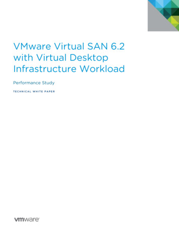
VMware Virtual SAN 6.2 with Virtual Desktop Infrastructure WorkloadPerformance of Hybrid Virtual SAN ClusterThe first experiment is on the 4-node hybrid Virtual SAN cluster where the desktop pool size in the cluster isvaried. We test with 400, 480, 500 and 520 virtual machines in the Virtual SAN 6.2 cluster and compare with a 6.1baseline. Virtual SAN performs very well in all cases: Group A scores are all under 1 second and Group B scoresare all under 6 seconds. The latency score numbers for 6.1 and 6.2 are still very similar. Then, we deep-dive to the500 virtual machine pool size case and discuss the Virtual SAN performance in detail. Please note that each hostin the 4-node hybrid cluster has 20 physical CPU cores that have hyper-threading enabled, and the 500 virtualmachine pool translates into 6.25 virtual machines per physical core, which is a good consolidation ratio for VDI.Each host in the Virtual SAN cluster has 1 disk group of 1 SSD and 4 magnetic disks.View Planner ScoresVirtual SAN results for the 500 virtual machine case are plotted in Figure 2. View Planner scores for both Group Aand B are very similar for Virtual SAN 6.1 and 6.2 as shown in Figure 2 (a). Virtual SAN 6.2 achieves this scoreeven though it has more work to do because of its software checksum feature that ensures data integrity, inwhich every read is verified against the checksum and every write introduces an extra checksum write.CPU UtilizationThe system and Virtual SAN CPU utilization in the cluster is shown in Figure 2 (b). Here we see that the CPUresource is close to saturation for both 6.1 and 6.2 under the workload. Virtual SAN 6.2 uses 0.3% more CPU in thecluster, that is 0.48 of a physical CPU core. This small increase is due to the calculation overhead of softwarechecksum introduced in Virtual SAN 6.2. Overall 6.2 provides data integrity protection for the workload at a verysmall cost.Guest I/O per SecondThe guest IOPs per host is shown in Figure 2 (c). On each host, Virtual SAN 6.1 has 750 read and 740 write IOPs,while 6.2 gives 650 read and 720 write IOPs. The IOPs number in the View Planner VDI workload has a small runto-run variation, but the slightly lower IOPs for 6.2 does not indicate a performance degradation since the latencyscore for 6.1 and 6.2 are very similar and both meet View Planner requirements.Guest Average LatencyFigure 2 (d) plots the average latency for all guest I/Os, and for read and write I/Os respectively. Virtual SAN 6.1has an average guest latency of 10.1ms but Virtual SAN 6.2 has 17.2ms. Looking at the read and write latency, itcan be inferred that the increase of average latency in 6.2 is from write I/Os. The average write latency climbsfrom 17.1ms to 29.6ms from Virtual SAN 6.1 to 6.2. The increase in write latency is the result of a scheduling quirkin the vSphere networking stack that manifests itself under high CPU utilization conditions (The VDI run has aCPU utilization close to 100%). However, even though the write latency is higher in Virtual SAN 6.2, the ViewPlanner Score of application latency still meets the requirement, for both group A of latency sensitiveapplications and group B of I/O intensive applications.The average read latency for Virtual SAN 6.1 and 6.2 are similar and both low (Virtual SAN 6.1 gives 3.2ms and 6.2gives 3.8ms). The low read latency is because the Content-Based Read Cache is doing a good job caching guestI/Os. The CBRC cache hit rate is constantly above 80% on all 4 hosts in the cluster during the steady state whilethe VDI workload is running.TECHNICAL WHITE PAPER / 8
VMware Virtual SAN 6.2 with Virtual Desktop Infrastructure Workload6GroupA120GroupB10099.54Total99.41VSANCPU Utilization (%)Latency (sec)5804603402120000.80.56.16.26.1(a) View Planner score for 500 VMs desktop pool size1000Read OpsWrite Ops8006.2(b) System and Virtual SAN CPU utilization in the cluster35Average LatRead LatWrite Lat30Latency (ms)25600IOPS2040015102005006.16.2(c) Guest IOPs per host6.16.2(d) Guest average latencyFigure 2. Virtual SAN performance on hybrid cluster for 500 VMs desktop pool size: (a) View Planner scores (b) CPUutilization (c) IOPs per host, (d) Guest average latencyImpact of DOM Client Read CacheThe DOM client read cache is enabled by default in Virtual SAN 6.2, and to illustrate its impact, the 6.2 NC run hasthe DOM client cache disabled. Figure 3 shows the results of 6.2 NC and compares them with Virtual SAN 6.1 and6.2. The View Planner Score for 6.2 NC is very similar to 6.1 and 6.2 as illustrated in Figure 3 (a) and meets thelatency requirement. The read latency results are shown in Figure 3 (b). Virtual SAN 6.1 has only CBRC, 6.2 hasboth CBRC and DOM client cache, and 6.2 NC has only CBRC.There are 2 points worth noting: For all the three cases, guest read latency is similar and lower than 4ms, but the DOM client read latency ismuch higher (more than doubled). We already know this is because CBRC is caching a majority of guestreads. We can also see that the DOM client read latency is also reduced when its cache is enabled. Comparing 6.2and 6.2 NC, 6.2 has DOM client cache and 6.2 NC doesn’t. Clearly 6.2 has a lower DOM client read latency of8.6ms while 6.2 NC has a higher value of 12.2ms. When the DOM client cache is enabled, the internal IOPs isalso reduced because cached reads can skip the entire Virtual SAN I/O stack.For this particular VDI workload, the effect of the DOM client cache is not showing up because the CBRC cache inthe View Storage Accelerator is already caching the reads very well.TECHNICAL WHITE PAPER / 9
VMware Virtual SAN 6.2 with Virtual Desktop Infrastructure Workload6GroupA14GroupBVSAN DOM Client104Latency (ms)Latency (sec)Guest1253286412006.1(a) View Planner Scores6.26.2 NC6.16.26.2 NC(b) Guest read latency and Virtual SAN client read latencyFigure 3. View Planner Scores and read latency comparison for DOM client cache disabled case on hybrid cluster for500VMsTECHNICAL WHITE PAPER / 10
VMware Virtual SAN 6.2 with Virtual Desktop Infrastructure WorkloadPerformance of All-Flash Virtual SAN ClusterIn this experiment, the VDI workload is exercised on the 4 node all-flash cluster. Different combinations of VirtualSAN 6.2 new features are used in the experiments. We test with 500, 540, 580, and 600 virtual machines in thecluster as the desktop pool size to represent the typical VDI environment that has a high consolidation ratio butdoes not sacrifice application performance. Virtual SAN 6.2 performs very well in all cases by meeting the ViewPlanner scores requirements for Group A and B applications. Next, we deep-dive to the 580 virtual machine poolsize case and discuss the Virtual SAN performance in detail. Each host in the 4-node all-flash cluster has 24physical CPU cores that have hyper-threading enabled, and the 580 virtual machine pool translates into 6.04virtual machines per physical CPU, which is a good consolidation ratio for VDI. Every host in the Virtual SANcluster has 2 disk groups, and each disk group has 1 caching SSD and 3 capacity SSDs. Please note this is not aconfiguration optimized for achieving lowest cost per VDI desktop virtual machine, but it represents a typical allflash Virtual SAN setup.View Planner ScoresFigure 4 shows the detailed results for 580 virtual machines to compare 6.2 new features. Figure 4 (a) shows theView Planner latency scores of Group A and B applications. Virtual SAN 6.2 performs well and meets ViewPlanner requirements. Furthermore, we can see
3 VMware Virtual SAN 6.2 with Virtual Desktop Infrastructure Workload Executive Summary