Transcription
C-band High and Extreme-Force Speeds (CHEFS)- Final Report -Ad Stoffelen1, Alexis Mouche2, Federica Polverari3,Gerd-Jan van Zadelhoff1, Joe Sapp4,5, Marcos Portabella3,Paul Chang4, Wenming Lin6 and Zorana Jelenak4,7Royal Netherlands Meteorological Institute (KNMI), De Bilt, The NetherlandsInstitut Français de Recherche pour l’Exploitation de la Mer (IFREMER), Plouzané, France3Institut de Ciències del Mar (ICM–CSIC), Barcelona, Spain4NOAA/NESDIS Center for Satellite Applications Research (STAR), College Park, MD, USA5Global Science & Technology (GST), Inc., Greenbelt, MD, USA6Nanjing University of Information Science and Technology (NUIST), Nanjing, China7University Corporation for Atmospheric Research, Boulder, CO, USA12EUMETSAT ITT 16/1661
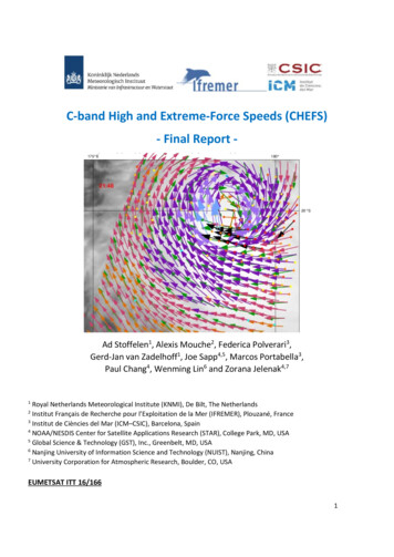
Front CoverASCAT-B scatterometer wind arrows in colour with an infrared satellite image (from Himawari)and numerical weather prediction model forecast winds from ECMWF as green arrows. Thescatterometer and model winds are from 28 December 2019 21:48, while the IR is from 21:30UTC. The scatterometer winds are coloured according to the Beaufort scale, winds up to 5 Bft.(10.7 m s-1) are in red, winds as of 6 Bft. are coloured as shown in the legend below. A blackarrow or flag indicates that the KNMI QC flag is set (MLE 18). The coloured dots give the valueof the Maximum Likelihood Estimator (MLE) which indicates how well an observation fits to theGeophysical Model Function (GMF). High MLE values indicate high spatial wind variability in theWind Vector Cell, WVC (from http://projects.knmi.nl/scatterometer/tile prod/tile app.cgi?).(c) EUMETSAT/KNMIAcknowledgementsEUMETSAT supported the CHEFS study, which provided resources to KNMI, ICM and IFREMERto lead and progress on the ocean winds community issue of an in-situ reference for satelliteand model calibration of extreme winds. Such study is only possible with access to uniformlyreprocessed wind data sets which were obtained from NOAA/NESDIS/STAR OSWT dropsondesand SFMR, ICOADS buoys, ECMWF buoy archive and ERA5 winds, ESA Sentinel-1 SAR andRadarSat SAR VV and VH data. In addition, we were informed by a NHC meeting in 2009 ontropical hurricane winds, discussions at several IOVWST meetings and many more informalcontacts with scientists knowledgeable in ocean wind measurements, Specifically, discussionswith Doug Vandemark, Jean Bidlot, Jim Edson, Lucia Pineau-Guillot, Ralph Foster and MarkBourassa specifically contributed to this report.Version 1:18 March 2020.Version 2:10 April 2020, Minor update figure 24.Version 3:3 June 2020,Correction of figure 39 and associated text, thanks to SébastienLanglade, DIROI/PREVI, Météo-France.2
CONTENTS1.INTRODUCTION . 42.DATA COLLECTION . 63.4.5.6.2.1.SFMR and dropsonde wind data . 62.2.Synthetic Aperture Radar and L-band radiometer. 92.3.ASCAT wind products reprocessed with ERA5 model winds . 122.4.Buoy wind description . 132.5.Effect of Stress-Equivalent Reference Winds . 132.6.Summary . 16SFMR CAL/VAL USING DROPSONDES . 173.1.SFMR/dropsonde collocation procedure . 173.2.Dropsonde winds . 183.3.Analysis of the WL150 dropsonde winds . 203.4.SFMR and dropsonde wind comparisons. 223.5.Summary . 28ASCAT/SFMR WIND COMPARISON . 294.1.ASCAT-related storm-centre estimates . 294.2.ASCAT/SFMR collocation approach . 314.3.ASCAT/SFMR wind comparisons . 344.4.Summary . 38ASSESSING BUOY WIND REFERENCE QUALITY . 395.1.Cwinds versus MARS buoy winds. 405.2.ASCAT/Buoy wind comparison . 425.3.Summary . 45SENTINEL 1 AND SFMR WIND COMPARISON . 466.1.C-band cross-polarization signal wind sensitivity . 466.2.Transects over Tropical Cyclones . 466.3.Signal sensitivity analysis with respect to ocean surface wind speed . 506.4.Saturation of VH signals . 556.5.Analysis against L-Band Brightness temperature. 596.6.Summary . 647.DISCUSSION AND CONCLUSIONS . 658.RECOMMENDATIONS . 689.REFERENCES . 6910. ACRONYMS . 733
1. INTRODUCTIONGlobal information on the motion near the ocean surface is generally lacking, limiting thephysical modelling capabilities of the forcing of the world’s water surfaces by the atmosphere(Belmonte and Stoffelen, 2019). This also limits our knowledge of the exchange of momentumacross the ocean-atmosphere interface, affecting meteorological and ocean applications(Trindade et al., 2019). A particularly pressing requirement in the Ocean Surface Vector Wind(OSVW) community is to obtain reliable extreme winds in hurricanes ( 30 m s-1) from windscatterometers, since extreme wind, storm surge and wave forecasts for societal warning are ahigh priority in nowcasting as well as in Numerical Weather Prediction (NWP).Scatterometers provide 10-m stress-equivalent winds (de Kloe et al., 2017), with a gridresolution of 12.5 km or 25 km. They have proven to be very effective for wind vector retrieval(Vogelzang et al., 2009). Over the years, improvements have been done on the development ofthe empirical Geophysical Model Functions (GMFs) in order to obtain more accurate windestimates with respect to in situ measurements. Scatterometer measurements are then largelyused for weather warning and forecasting, climate monitoring, research on processes, oceanforcing and air-sea interaction. Indeed, C-band scatterometers have the capability to provide allweather measurements, including in extreme wind conditions. However, developing andverifying wind scatterometer processing algorithms for high and extreme winds is challenging,since in situ wind measurements are scarce and they may be hazardous and unreliable.Moreover, theoretical statistical descriptions of the high-wind ocean surface, where patchyfoam, droplets, spume and wave breaking occur are much simplified, while the microwaveinteraction on cm scales is rather complex.In this framework of the Eumetsat-funded “C-band High and Extreme-Force Speeds (CHEFS)”project, the Koninklijk Nederlands Meteorologisch Instituut (KNMI), the Institut de Ciències delMar (ICM-CSIC) and the Institut Français de Recherche pour l'Exploitation de la MER (IFREMER)aim at assessing the extreme wind capabilities of the next generation of C-band windscatterometers on-board Metop Second Generation (SG), in order to provide reliable extremeocean surface vector winds information in open ocean and marine coastal regions, wheregenerally limited in-situ measurement capability exists. Three main objectives have beenproposed in this project: (i) improving the understanding of satellite remote sensing of highextreme wind conditions over ocean; (ii) the definition of spatial scaling issues and relatedconsequences for product sample resolutions and validations approaches; (i) understanding thecross-polarization contribution to the high-extreme winds.To this end, an important goal within CHEFS is to provide an appropriate and consolidated highand extreme-wind reference data set at scatterometer scales, based on in-situ wind references.This reference is crucial for purposes of scatterometer calibration and validation. Moored buoydata are generally used as absolute reference to calibrate the GMFs, however, for very high andextreme winds above 25 m s-1, moored buoys may not be reliable. Moreover, controversy existsin the OSVW satellite community on the quality of moored buoys above 15 m s-1 rather than 25m s-1 (e.g., Pineau-Gouillot et al., 2018). Therefore, collaboration has been sought with theOcean Surface Winds Team (OSWT) at the National Oceanic and Atmospheric Administration(NOAA)/National Environmental Satellite, Data, and Information Service (NESDIS)/Center forSatellite Applications and Research (STAR) (hereafter as NOAA/NESDIS/STAR OSWT) to haveadditional high and extreme winds reference data sets. The OSWT routinely fly into hurricanes4
and extratropical cyclones and deploy GPS drop-wind-sondes (also known as simply dropsondes)obtaining wind profiles. In addition, they operate dedicated microwave instrumentation on theaircraft to obtain detailed wind patterns in hurricanes, such as the Stepped-FrequencyMicrowave Radiometer (SFMR).The present report finalizes the CHEFS project. In particular, several wind data sets have beencollected, i.e., (i) different types of moored buoy data; (ii) reprocessed SFMR 10-m winds, from2008 to 2018; (iii) estimated 10-m dropsonde winds, from 2009 to 2018, along with thecorresponding raw/quality-controlled wind profiles; (iv) reprocessed ASCAT-A 10-m winds at12.5 km grid resolution, from 2007 to 2017; (v) the latest European Centre for Medium-RangeWeather Forecasts (ECMWF) fifth reanalysis dataset ERA5 from 2007 to 2017, and (vi) SyntheticAperture Radar (SAR) winds from Sentinel-1 and RadarSat. The collected datasets are discussedin Section 2 of this report. A comprehensive SFMR wind statistical analysis using dropsonde dataas reference is presented in Section 3. The impact of the so-called WL150 algorithm used tocompute the dropsonde 10-m winds on the SFMR/dropsonde statistics has been also evaluated.An SFMR winds re-calibration has not been performed at this time, but rather suggestions andoutliers to be taken into account when comparing dropsonde and SFMR winds are presented.Subsequently, the ASCAT and SAR high-wind performance and calibration are investigated withrespect to collocated SFMR winds in Section 4 and 6 respectively. The quality of buoy windsbetween 15 m s-1 and 25 m s-1 is thoroughly evaluated in Section 5. ASCAT surface winds aremoreover used as a reliable and stable calibration reference to bridge buoy andSFMR/dropsonde collocations, to allow indirect inter-comparison between such datasets at thescatterometer scale, as sufficient direct collocations of buoy and dropsonde winds were notavailable. Some conclusions may be drawn from SAR and L-band radiometer (SMAP)comparisons. The inconsistencies between buoy and SFMR/dropsonde winds together withmore general conclusions are then discussed in Section 7 and, finally, the recommendations ofthis study can be found in section 8.5
2. DATA COLLECTION2.1.SFMR and dropsonde wind dataThe SFMR and dropsonde datasets are provided by the NOAA/NESDIS/STAR OSWT. Thesedatasets have been acquired by the many NOAA WP-3D and U.S. Air Force Reserve Command(AFRC) flights over several hurricane seasons. For each flight, the hurricane hunters’ aircraftcrosses the storm centre several times, acquiring both SFMR sea surface wind and rain alongwith wind profiles from the Global Positioning System (GPS) dropsondes. An example of theSFMR wind speed variation along a flight trajectory as well as a wind profile from a dropsondelaunched from the same flight are shown in Figure 1(a) and Figure 1(b), respectively. As can beseen from the SFMR wind variation, during each storm cross, the wind intensity alternativelygoes from high to low speeds and the wind minima usually move during this time, identifyingthe movement of the storm.(a)(b)Figure 1. (a) Wind variation during the NOAA hurricane hunters flight experiment on August 18th, 2009. Wind dataare obtained from SFMR measurements. (b) Dropsonde wind profile acquired from NOAA hurricane hunter duringthat same flight experiment.A third dataset is also collected from the Imaging Wind and Rain Airborne Profiler (IWRAP) onboard the NOAA P-3 flights. However, this instrument only operates on a subset of these flightsdepending on whether or not the instrument space has been provided for the whole hurricaneseason and whether or not the storm is of interest. Due to the limited data availability, thisdataset has not been used in this work. However, it is available for future analysis.For this study, ten years of SFMR wind and rain retrievals reprocessed by NOAA/NESDIS/STAROSWT have been collected from 2009 to 2018. These data have been reprocessed using a newGMF that corrects an approximate 10% low bias observed in the SFMR wind retrievals between15 and 45 m s-1 with respect to dropsondes [Sapp et al., 2019], i.e., the so-called WL150 windsas discussed later. SFMR is a passive nadir-looking instrument that measures the brightnesstemperature (𝑇𝑇𝐵𝐵 ) of the ocean surface at six C-band frequencies. In order to ensure that the 𝑇𝑇𝐵𝐵values measured during the flight are accurate, an in-flight ocean calibration is alwaysperformed prior to each flight campaign. For each channel, such ocean calibration aims toadjusting few of the instrument internal temperature coefficients forming the 𝑇𝑇𝐵𝐵 calibrationequation, in order to reflect the actual conditions. However, errors in the definition of thesecalibration coefficients may occasionally occur, leading to differences between the SFMRmeasured 𝑇𝑇𝐵𝐵 values and the corresponding 𝑇𝑇𝐵𝐵 values predicted by the GMF, i.e., the so-calledtuning error. The NOAA/NESDIS/STAR OSWT has developed a 𝑇𝑇𝐵𝐵 bias correction routine in orderto correct for these differences. Such correction is applied to the measured 𝑇𝑇𝐵𝐵 and the corrected6
value is then used in the wind retrieval process. More details can be found in Sapp et al. (2019).The SFMR dataset used for the present study has been inspected by the NOAA/NESDIS/STAROSWT to ensure that they were good in terms of instrument calibration and wind retrievals. Inparticular, they have excluded those data whose 𝑇𝑇𝐵𝐵 values was not considered as reliable,because of: (i) 𝑇𝑇𝐵𝐵 differences amongst the six channels higher than 2K, suggesting possibleerrors in the 𝑇𝑇𝐵𝐵 calibration equation; (ii) presence of high amount of noise in the 𝑇𝑇𝐵𝐵 channels;(iii) possible instrument instability (visible in few SFMR flights of 2008, but which has been fixedsince then). As shown in Sapp et al. (2019), the standard deviation of the SMFR wind speed errorwith respect to dropsondes is typically 3-4 m s-1 for wind speed between 15-40 m s-1 in low rain,while biases are below 1 m s-1 with respect to WL150.The wind retrievals are provided at a frequency of 1 Hz. Note that most NOAA P-3 flights havemore accurate geolocation information than AFRC flights. As it can be seen in Figure 2, SFMRdata points from the AFRC flight on June 20th, 2019 are geolocated at a grid resolution of 0.01deg. This is because AFRC geolocation (latitude/longitude) information is archived in floatingnumbers with only two decimals. As such, assuming a flight speed of about 100 m s-1 and anSFMR sampling rate of 1 Hz, about 10 SFMR data points are assigned to the same lat/lon positionin AFRC flights. Also, depending on the flight orientation, the SFMR data points are grouped overtwo apparent parallel tracks, whereas in reality there is only one single track distributed. Thisleads to a geolocation error of / 0.005 deg, which should be taken into account when usingAFRC data. Note that the geolocation error is very much reduced in NOAA P-3 flight data, sincea higher precision geolocation information (floating-point numbers with four decimals) is kept.A quality control (QC) flag is available in the wind products in order to discriminate the validwind solutions from those questionable or invalid.Figure 2. SFMR raw data outlined by boxes, from AFRC flight on June 20th, 2017.GPS dropsondes are launched from the hurricane hunters’ aircraft to measure profiles of windspeed, direction, pressure, temperature and relative humidity from the moment they are7
launched until they reach the ocean surface (Hock et al., 1999). The dataset used in this analysiscovers the period between 2009 and 2018 according to the SFMR dataset. These data have beenfiltered by the NOAA/NESDIS/STAR OSWT in such a way that only the dropsondes outside thehurricane eyewall and in tropical cyclone conditions have been included. In addition, they referto dropsondes relevant for SFMR-dropsonde collocation purposes. Details on the criteria usedto filter the data can be found in Table 2 of Sapp et al., (2019).The data have been provided in two different forms: on the one hand, the entire wind profile ofeach dropsonde and, on the other hand, the corresponding estimated 10-m winds. As it will bediscussed in Section 3.2, the dropsonde 10-m winds are estimated by an averaged windcomputed from the corresponding wind profile [Franklin et al, 2003, Uhlhorn et al., 2007]. Boththe raw and the QC-ed wind profiles have been provided. The latter are obtained by processingthe raw profiles using the NCAR’s Atmospheric Sounding Processing Environment (ASPEN)software, which systematically detects and removes the incorrect measurements. After exitingthe aircraft, the soundings usually undergo an extreme change, so that all the sensors need timebefore they settle in the new environmental conditions and they start acquiring validmeasurements. ASPEN usually filters out these invalid points. Note that the dropsonde profilesof 2018 have been processed with a new release of ASPEN and the output format sligthly differsfrom the previous one. Due to time constraints, the developed data reader could not beadapted, so that the wind profiles of 2018 could not be used at this time and will be included infuture analyses.The the time of the first reliable measurement is assigned to the resulting QC-profile asdropsonde launch time and this time may differ from the actual launch time. On the other hand,the actual information of the launch time is generally stored in the raw profiles. As aconsequence of such time difference, the SFMR point at the dropsonde launch time stored inthe QC-profiles (hereafter as SFMR-LQC) may be displaced with respect to the SFMR point at theactual lanch time (hereafter SFMR-LRAW). An example is shown in Figure 3. A transect of the SFMRflight on August 25th, 2011 is displayed along with the positions of a dropsonde launched duringthat flight. It can be seen that ASPEN has filtered quite a few dropsonde data points from theraw profiles (black dots). The launch time in the QC-profile is 39 sec apart from the time in theraw profile. This results in a displacement between SFMR-LQC and SFMR-LRAW of about 5.2 km atan aircraft speed of 133 m s-1. These time differences are taken into account here when usingthe launch time for dropsonde/SFMR collocation purposes (see Section 3.1).A total of 2,174 estimated dropsonde 10-m winds are available. However, 10% of thesedropsondes do not have the corresponding QC/raw profile available in our dataset. In addition,7% of the dropsondes do not have the corresponding SFMR flights, which may have beenremoved from our dataset because of calibration issues or available wind speeds lower than 15m s-1, where SFMR is not reliable. As such, a total amount of 1,804 dropsonde profiles are usedin the dropsonde/SFMR wind comparison. Note that, when carrying out dropsonde windanalysis which does not involve the use of SFMR winds or raw dropsonde profiles, we couldenlarge the number of used dropsondes up to 1,983 out of 2,174 available.8
Figure 3. Transect of SFMR data during the NOAA flight on August 25th, 2011. Both the raw (black dots) andthe QC profile (pink) of a dropsonde launched during the same flight experiment are shown. Both SFMRpoints at the launch time stored in the QC-profile (red cross) and in the raw profile (blue cross) are outlined.2.2.Synthetic Aperture Radar and L-band radiometerSynthetic Aperture RadarDespite having a single antenna, existing C-band SAR systems can acquire data in both co- andcross-polarization. Consequently, they can provide valuable data before the launch of theMetop-SG scatterometer SCA in order to improve our understanding of the C-bandbackscattered signal and prepare the mission. In particular, its dual-polarization capability allows to directly compare the sensitivity of co- and crosspolarized backscattered signal to ocean surface wind speed and direction but also otherphenomena such as intense rainfall that can lead to issues for ocean surface windretrieval. its high resolution allows to analyse the impact of the resolution in order to describe thedynamic of strong but « small » phenomena such as Tropical Cyclones. As a matter of fact,the capability of a sensor to accurately measure the maximum wind speed of a TC isdirectly related to its spatial resolution and the TC size.In the following, Sentinel-1 and Radarsat-2 SAR data are introduced for these purposes.The Sentinel-1 mission (S1) is part of the operational European Copernicus program spacecomponent. S1 is a constellation of two satellites (S1-A and S1-B units). Both Sentinel-1A and 1B carry a C-band Synthetic Aperture Radar (SAR) and continue previous European ERS andENVISAT SAR missions. Sentinel-1A & -1B were launched in April 2014 and 2016 respectively.They have four exclusive imaging modes: Interferometric Wide swath (IW), Extra Wide (EW)swath, Strip Map (SM) and Wave (WV) modes. The IW swath is 250 km wide and coversincidence angles from about 30 to 46 degrees. When processed into Level-1 (L1) GRDH (Ground9
Range Detected High resolution), IW Sentinel-1 products have a resolution of about 20 m inrange (across-track) and 22 m in azimuth (along-track). The EW swath is 400 km wide and coversincidence angles from about 30 to 46 degrees. When processed into L1 GRDH, EW Sentinel-1products have a resolution of about 50 m in range (across-track) and 50 m in azimuth (alongtrack).Tasking SAR with respect to the hurricane tracks forecast is required to jointly maximizeacquisitions over TCs and mitigate the impact on the whole mission acquisition plan. This impliesto solve potential conflicts between users regarding the duty cycle along the orbit and theacquisition modes to be used over a given area of interest. Since 2016, ESA set up specific S1acquisition campaigns to test the instrument capabilities for mapping, at very high resolution,extreme (TC) ocean wind conditions. These campaigns of dedicated acquisitions are named asSHOC, for Satellite Hurricane Observations Campaign. Fully coordinated as for the hurricanewatch program approach (Banal et al., 2007), SHOC campaigns help maximizing the number ofSAR acquisitions for both Copernicus/ESA Sentinel-1 and MDA Radarsat-2 missions. For thisstudy, the strategy to collect the data over TC includes two different approaches. (i) As part ofSHOC, we collect the data through acquisitions requests for both Radarsat-2 and Sentinel-1missions respectively to MDA and ESA. These requests are based on 5-day forecasts of thehurricane track and satellite orbit. This approach requires great flexibility for data provider. (2)We also analyse the SAR data archives and the maximum wind speed with respect to thehurricane Best-Tracks database to find observations over TC in the past data. The periodconsidered for the archive analysis is from 2015 and 2017. Radarsat-2 data from the archivehave been analysed in cooperation with Prof. Biao Zhang from NUIST (Nanjing, China).To date, SHOC is still on-going. Thanks to this campaign, after the 2018 summer TC season, atotal of 194 acquisitions over TC eyes are available, yielding to an unprecedented SAR TCcollection over 5 distinct basins. Recently, the first acquisitions of the North Indian Ocean havebeen obtained.Figure 4. Composite view of TC cases for each geographical zone, where basin locations are indicated inthe global map (centre bottom panel). Acquisition positions from Best-Tracks are displayed for each TC,where colours depict intensities with respect to Saffir-Sampson scale. Markers are stated for TC positionswith measurements. Red square: SAR measurements only; Green diamond: sequential measurements ofSAR and SFMR.10
After the filtering steps (partial TC eye for instance), 161 snapshots corresponding to 72 differenttropical systems in the period 2015-2018 can thus be analysed. Figure 4 synthesizes the S1 dataset. For each storm, the 6-hour Best-Track locations with corresponding storm intensity (colours)are indicated. Specific markers highlight the collocation opportunities: a red square when onlySAR is available and a green diamond, when simultaneous SAR SFMR measurements co-exist.Because aircraft measurements are restricted to North American basins, with a majority in theAtlantic and a few paths in the Eastern Pacific, collocations with SFMR count for only 13% of thedata set, with respectively 23 and 6 flights for the Atlantic and East-Pacific. 70% of the Atlantichurricanes are actually covered. The intensity histogram illustrates the spectrum of TCintensities. Unlike most of the previous SAR-based studies, all Saffir-Simpson scale intensitiesare sampled.L-band Radiometer (SMAP)Both the VH NRCS and L-band radiometer returns depend on wind speed, with little ancillarysensitivity to wind direction, and are potentially capable of retrieving extreme winds. Hence, itis useful to compare both ocean returns, which is possible by collocating S1 SAR and the NASASoil Moisture Active Passive (SMAP) L-band radiometer data (https://smap.jpl.nasa.gov/).The L-band radiometer on-board SMAP scans a wide 1000-km swath with a spatial resolution of40 km. The L-band radiometer measures the four Stokes parameters, Tv , Th , T3 , and T4 , at afrequency of 1.41 GHz with a surface incidence angle of approximately 40 . TB,rough is the quantityused in by Reul et al. (2012; 2016), Yueh et al. (2016) and Meissner et al. (2017) to relate oceansurface L-band emission and ocean surface wind speed. In order to estimate TB,rough from SMAPantenna measurements, radiometer calibration is applied, and several contributions to theantenna temperature are removed or filtered such as radio frequency interferences, extraterrestrial contributions (galaxy, sun, etc.), and faraday rotation across the ionosphere(Piepmeier et al., 2016). Then atmospheric corrections are performed to estimate brightnesstemperature emitted by the ocean surface (TB,surface). At last, the brightness temperature of theflat ocean surface, a function of the sea surface salinity (SSS) and sea surface temperature (SST),is subtracted from TB,surface to get the residual brightness temperature TB,rough. To estimateTB,surface, we used external monthly SSS from World Ocean Atlas (WOA) 2009 and EuropeanCentre for Medium range Weather Forecasting (ECMWF) 3-h forecast SST.SMAP L-band radiometer can measure the same target from two different azimuth angles,thanks to the rotating scan of the antenna. TBh,rough and TBv,rough measured forward and afterwardof the SMAP satellite position are averaged to reduce directional variation. In this report, weconsider the first Stokes parameter (TBh,rough T Bv,rough)/2.0 for analysis against Sentinel-1 NRCS.The spatial resolution of original NASA level 1B SMAP data is about 40 km, while the reprocessedSMAP product used here is mapped onto a global grid with spatial resolution of 0.25 .To perform accurate analysis of Sentinel-1 NRCS and SMAP TB,rough, we collocate SMAP TB,roughwith Sentinel-1 NRCS, and IMERG rain rate (rain product from NASA) as illustrated in Figure 5.For spatia
reprocessed wind data sets which were obtained from NOAA/NESDIS/STAR OSWT dropsondes and SFMR, ICOADS buoys, ECMWF buoy archive and ERA5 winds, ESA Sentinel-1 SAR and RadarSat SAR VV and VH data. In addition, we were informed by a NHC meeting in 2009 on tropical hurricane winds, discussions at several IOVWST meetings and many more informal