WIXLIB

May 31, 2018 18:6ws-rv961x669Book TitleStandard Problems in Micromagneticsporterpage 55interpretation and understanding. The LLG form (1) is most commonly used toinvest the equation with physical meaning, while analysis of the LL form (7) canoften reveal useful information more easily. The LL form can also be easier to workwith numerically because it defines dM/dt explicitly in terms of M and H.In the LLG formulation, we can imagine the degree of damping to increase without limit, but it’s clear when we transform back to the LL form that an arbitrarilylarge α simply leads to shrinking values for both γ̄ and λ. (The maximum value forthe ratio α/(1 α2 ) is 1/2, which occurs at α 1.) That is, an increasingly viscoussystem simply grinds to a standstill. Practical scenarios include only values of αless than or equal to 1. Within those limits, the particular value of α appropriateto a calculation is a property of the material under simulation.In either LLG or LL form, it is clear that dM/dt is orthogonal to M. Thismeans that the pointwise magnitude of the magnetization does not vary over time, M(r, t) Ms (r) for all t. This is one of the fundamental constraints in canonicalmicromagnetics.For the purposes of analyzing the magnetization dynamics, the LL form is somewhat simpler than the LLG form because the two terms on the right hand side ofthe LL equation are not only orthogonal to M but also orthogonal to each other.The M H term is orthogonal to H and therefore describes precession aboutH. Moreover, if we view the energy W as a surface over the space of magnetization configurations, then by (4) we see that H is aligned with the downhill (lowerenergy) direction on that surface. Therefore, motion perpendicular to H is energy neutral. Conversely, it follows from the vector triple product identity thatM H M/Ms2 H (M · H)M/Ms2 , which is the projection of H onto thespace orthogonal to M. In other words, the damping term in the LL equation isin the direction of the component of H compatible with the magnetization normconstraint, and so motion in this direction tends to align M with H and lowers theenergy.It is clear from the LL form that stationary configurations, where dM(r)/dt 0for all r, occur exactly when M(r) H(r) 0 (or equivalently, M(r) is parallel toH(r)) for all r. In this case both terms on the right hand side of (7) are individuallyzero. It follows from (4) that stable stationary configurations correspond to localenergy minima. Therefore, we see that terminating configurations of LLG trajectories are local minima of the energy. For many purposes the complete dynamics ofthe magnetization are not important, so long as these energy-minimizing magnetization states can be determined. In such cases direct energy minimization, usingfor example conjugate-gradient methods, can be many times faster than solving theLLG equation.Energy minimization is at the core of the technique known as quasi-static micromagnetics. A local energy minimum is computed at one applied field held staticover the minimization step. After the equilibrium configuration is found the appliedfield is changed slightly (stepped) and then a new energy minimizing configuration

May 31, 2018 18:66ws-rv961x669Book TitleporterD. Porter & M. Donahueis sought starting from the previous energy minimum. This process is repeatedacross the full desired range of applied field. This method is at the heart of the firsttwo µMAG Standard Problems. The third µMAG Standard Problem also directlyaddresses the task of energy computation.Of course, there are many instances where the full magnetization dynamics areimportant, in which case there is no alternative to solving the LLG equation for thetime varying magnetization. The fourth and fifth µMAG Standard Problems are ofthis class.The LLG equation is the most commonly encountered representation of magnetization dynamics for micromagnetics, and it is also the most basic. Variousextensions have been proposed which can more faithfully reproduce experimentalobservations in some circumstances. For example, the damping factor α in theLLG equation is a phenomenological term representing the simplest way to modelenergy loss in a dynamic magnetic system. More complex, non-isotropic and nonlocal models of damping are possible.11–13 More radically, the norm constraint M(r, t) Ms (r) for all t can be relaxed with the introduction of a restoringforce that instead causes M(t) to only tend toward Ms . This property underpins the Landau-Lifshitz-Bloch (LLB)14–17 and Landau-Lifshitz-Baryakhtar (LLBar)18–20 equations. New physics, such as the spin-torque effect, can be introducedwith the addition of the Slonczewski spin-transfer torque term (LLGS),21–25 whichis the subject of the fifth µMAG Standard Problem.Each of the µMAG Standard Problems is presented in detail in Sec. 4. Toprepare for that presentation we first examine the energy components that makeup a micromagnetic simulation.2.2. Magnetic Energy ComponentsThe LLG equation predicts the dynamics of magnetization as a function of the magnetization configuration and the total effective field H. At each point in space, H(r)can be described as a sum of magnetic fields arising from different sources. The fourfundamental sources in micromagnetics are the anisotropy energy, the quantummechanical exchange energy, the self-magnetostatic (dipole-dipole) energy, and theZeeman energy. Some of these components depend only on material properties andthe magnetization configuration M. For those terms H(r) may depend on M at onlythe point r itself (e.g., anisotropy), on M in a small neighborhood of r (exchange),or on M globally across the entire volume of the simulation (self-magnetostatic).Other components of H may be independent of the magnetization configuration M.These represent the influence of the environment outside of the material of interest,and are represented as applied fields (Zeeman).page 6

May 31, 2018 18:6ws-rv961x669Book TitleporterStandard Problems in Micromagneticspage 772.2.1. Anisotropy EnergyOne of the simpler energy source terms is the anisotropy energy. It is the tendencyof electron spins to interact with the atomic structure of the material in such away that magnetization in certain directions is favored over others. The anisotropyenergy is defined to prefer favored directions with an energy penalty for movingaway from the such directions. As an example, a material with a single favoreddirection along an axis determined by unit vector u, may be represented by theenergy term 2 ZMd3 r.(10)·uWK K M VSuch a material is said to have a uniaxial anisotropy. The anisotropy is characterizedby the value of anisotropy energy density K in units of joules per cubic meter(J/m3 ). The values of K and u may vary spatially. If K 0 then u is an easy(energetically preferred) axis for the magnetization. If K 0 then u is a hardaxis, that is, it is energetically favorable for the magnetization to lie in the planeorthogonal to u (which is known as the easy plane for magnetization).It follows from (4) that the anisotropy field corresponding to (10) isHK 2K(M · u) u.µ0 M 2(11)Other anisotropies favoring multiple axes, or having higher-order dependencies,may be specified by analogous energy terms.26–29 In many of these cases, thecrystalline structure of the material is reflected in the energy term, and it is thenknown as the magneto-crystalline anisotropy. As an example, cubic anisotropy canbe represented byZ KMx2 My2 Mx2 Mz2 My2 Mz2 d3 r(12)WK,cubic 4 M Vwith associated fieldHK,cubic 2K Mx My2 Mz2 ex My Mx2 Mz2 ey4µ0 M Mz Mx2 My2 ez .(13)2.2.2. Exchange EnergyMicromagnetics is conceived as a continuum theory. The vector fields are taken to becontinuous functions of continuous space. As a physical matter, magnetization arisesfrom the quantum mechanical exchange interaction. In ferromagnetic materials, theeffect of this quantum phenomenon is to align magnetic moments of electrons withthe magnetic moments of other nearby electrons. This leads to the formation ofmagnetic domains within magnetic materials. In continuum micromagnetics, anexchange energy term that penalizes large spatial rates of change in magnetization

May 31, 2018 18:68ws-rv961x669Book TitleporterD. Porter & M. Donahueconfigurations achieves the same end. A conventional formulation for exchangeenergy isZ A 222 M M M d3 r,(14)Wexch xyz2V M where A is an exchange coefficient measured in joules per meter (J/m). This canalso be written as30 2 Z M 2M 2MAM· d3 r.(15)Wexch 2222 M x y zVThe corresponding expression for the exchange field is 2 2A M 2M 2MHexch µ0 M 2 x2 y 2 z 2(16)Since these expressions are founded on spatial derivatives of the magnetization,a set of suitable boundary conditions must be defined. When the boundary of ourvolume of interest corresponds to the boundary separating a magnetic material fromspace where magnetization is zero, the natural Neumann constraint M 0(17) ntakes hold, while in other situations, other choices are possible.30More complex forms for the exchange interaction are sometimes used, includinganisotropic variants.312.2.3. Self-Magnetostatic EnergyAny spatial pattern of magnetization gives rise to a magnetic field Hdemag as determined by the simultaneous solution of the relevant Maxwell equations, · Hdemag · M, Hdemag 0.(18)(19)The quantity Hdemag is known by many names, including “self-magnetostatic field,”“dipole-dipole field,” and “demagnetizing field.” The effects of this field are atwork when matters of shape anisotropy are considered. If we imagine our continuum representation of magnetization as an approximation to a collection of discreteelementary magnets, the magnetostatic field is the field required to represent thesum of the dipole-dipole interactions of the collection of magnets. For a volume ofinterest V bound by a closed surface S with normal vector n, the magnetostaticfield is computed asZZ1r r0 3 01r r0 2 0000Hdemag (r) · M(r )dr n·M(r)d r (20)4π V r r0 34π S r r0 3The demagnetizing field at each point is seen to be a function of M throughoutthe volume of interest. This is a field describing long-range interactions, unlikethe other energies that describe interactions in a local volume. The consequence ispage 8

May 31, 2018 18:6ws-rv961x669Book TitleporterStandard Problems in Micromagneticspage 99that the largest part of the computational burden in a micromagnetic model is thecalculation of the self-magnetostatic fields and energies.While the exchange energy favors the formation of magnetic domains (i.e., regions of generally uniform magnetization), the magnetostatic energy tends to favoranti-parallel alignments that break up domains. The task of micromagnetics is often the computation of what equilibrium arises from these competing tendencies.Given the quantity A in J/m which characterizes the exchange energy, and the saturation magnetization Ms M in A/m characterizing the magnetostatic energy,the expressions2A(21)lex µ0 Ms2is a length in meters. This quantity is known as the (magnetostatic) exchange lengthof the material; it is typically around 5 nm for the more common magnetic materials. For magnetically soft materials (i.e., ones with small anisotropy constant K),this is the scale of spatial features found in energy minimizing magnetization configurations, and so provides a guide to the required spatial resolution of discretizationsfor micromagnetic simulations. For magnetically hard materials (those with large K ), another distance of interest is the magnetocrystalline-exchange length, givenbyrA.(22)lex,K KHere K is in J/m3 , so again this is a length in meters. Typically the simulationdiscretization should be chosen smaller than either exchange length; in other words,the smaller exchange length is the controlling length scale.2.2.4. Zeeman EnergyThe effect of magnetic fields arising from outside the materials in the volume ofinterest is represented in a term known as the Zeeman energy. Since their origin isfrom outside the system, they enter the computation as inputs, typically as an applied field Happ specified by magnitude and direction within the volume of interest.The relation between the energy and field is simplyZWapp µ0Happ · M d3 r.(23)VThese four energies, anisotropy, exchange, self-magnetostatic, and Zeeman, arethe most commonly encountered energy sources in micromagnetic simulations. However, it is straightforward to include additional energy/field terms to representother effects, such as thermal agitation,32–36 magnetoelastic behavior,37–39 or theDzyaloshinskii-Moriya interaction (DMI).40–43

May 31, 2018 18:610ws-rv961x669Book Titleporterpage 10D. Porter & M. Donahue2.3. States, Energies and Solver RequirementsThe sum of the four magnetic energy terms, anisotropy, exchange, magnetostatic,and Zeeman, form the foundation of micromagnetic simulations. For many values ofthe parameters identifying the environmental state, and the relevant properties ofthe simulated materials, multiple local minima of the magnetic energy are possible.Which minimum is to be chosen is controlled by the trajectory by which it is reached,which in turn reflects the history of environmental states. This feature of themicromagnetic model provides for a representation of hysteresis in the calculationmatching the hysteresis of magnetization observed in physical magnetic materials.The ability to store in the magnetic state of a material a record of the history of itsenvironment is precisely what makes magnetic materials interesting as a buildingblock for information storage technologies.Magnetic materials are often characterized by their bulk properties. Given anyset of parameter values characterizing material properties that govern the internalmagnetic energy terms, we can find an applied field of sufficient magnitude so thatthe Zeeman energy term overwhelms all the others. In that extreme, in principle,only a single local minimum of magnetic energy remains, the state in which magnetization is nearly uniformly aligned with the applied field. In physical terms,we can say that we have placed the material in a state of saturation. From thesaturation state, the magnitude of applied field may be reduced to zero, and thenraised to a saturation value in the opposite direction and back again. In response,the bulk magnetization of the material will pass from a positive value of saturationto a negative value of saturation and back again, in a sequence of states knownas the major hysteresis loop of the material. The micromagnetic model is capableof representing and computing this behavior. Key points of the major hysteresisloops are of interest in characterizing materials. The value of bulk magnetizationremaining when the applied field has been reduced to zero is known as the remanent magnetization. The magnitude of reversing applied field necessary to reducethe bulk magnetization to zero is known as the coercive field, or coercivity. A validity check that a micromagnetic model properly represents a physical material isto see whether computed values of remanence and coercivity match with physicalmeasurements.Any software claiming to be a micromagnetic solver will have the ability to compute the energies and fields so far described, represent magnetization states, acceptas inputs the material properties and initial and boundary conditions needed todescribe the simulation, and output some suitable representation of the magnetization states computed as equilibrium states. The set of computations might be anumerical solution to LLG, or might be an energy-minimization approach to findingthe same set of energy minima states, as appropriate to the needs of the user.

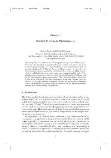
May 31, 2018 18:6ws-rv961x669Book TitleStandard Problems in Micromagneticsporterpage 11113. Obstacles to Clear Communication and Accurate ResultsWhile there is broad common understanding in the foundations of micromagneticmodeling just described, there are also many points where variations of understanding or approach may lead to miscommunication.The study of magnetism has a long history that has been characterized by theuse of multiple systems of units. Although the SI system is becoming predominant,other systems, notably the Gaussian system, are still in use and are prevalent inhistorical works. This is a particular challenge because the different unit systemsare not mere rescalings of one another, but the fundamental relations differ. Forexample, in SI we have B µ0 (M H), with B in T and M and H in A/m. In theGaussian system this renders as B H 4πM with H in Oe and B and 4πM inG. The implication is that we not only have to contend with different sets of units,but with different equations representing the same physical phenomena. Withoutcare, it is a common error to interact with software built on one understanding, yetselect input values for it founded on a different incompatible understanding.Another source of potential disagreement among the solutions of different micromagnetic solvers arises when the equations to be solved are mapped into representations on which to perform computations. The elements of the model equations arecontinuous vector and scalar fields, conceived at arbitrary precision and resolution.When we enlist computation to solve our equations, those idealized componentsmust be reduced to one or another representation as collections of limited precisionfloating-point numbers held in limited stores of memory. While there are manysensible ways to do this, each brings with it limitations on the boundaries of application. The question must always be asked whether any representation, or anyalgorithm carried out on that representation, continues to make sense when appliedto any particular problem as posed. Because different choices of representations andalgorithms carry with them different limitations, it is not desirable to dictate oneor another choice. It is better to let different research teams explore the differingcapabilities of different choices. At the same time they must be assigned the burdenof reporting the computed results in a common language that can be shared beyondthe bounds of their particular assumptions.There are sometimes also subtle issues surrounding implicit assumptions. Forexample, consider how one might specify the initial state of a simulation. Whenwe speak of a part being magnetically saturated, we envision the magnetizationas being uniformly oriented in the direction of an applied field. But unless thepart is ellipsoidal, exactly uniform alignment is not an equilibrium state. Rather,the self-magnetostatic field will cause some canting of the magnetization near partedges and corners, as illustrated in Fig. 1. The canting will diminish as the appliedfield is strengthened, even to the point where it is visually difficult to distinguishbetween the various states, but nonetheless the differences will reemerge when thefield is reduced and can influence subsequent magnetization activity. This meansthat specifying that a simulation begin in a saturated state is not sufficient to pin

May 31, 2018 18:6ws-rv961x669Book Title12porterpage 12D. Porter & M. DonahueHSplayedFig. 1.“S”“C”Three nominally saturated magnetization states.down subsequent behavior. Even identifying all the available equilibrium states isa non-trivial problem, a point demonstrated in Standard Problem 3.We should point out too the difficulties posed by symmetric states, such as the“splayed” state in Fig. 1. These frequently are or devolve into saddle points on theenergy surface. There are multiple, equally-valid

May 31, 2018 18:6 ws-rv961x669 Book Title porter page 1 Chapter 1 Standard Problems in Micromagnetics Donald Porter and Michael Donahue National Institute of Standards and Technology, 100 Bureau Drive, Stop 8910, Gaithersburg, MD 20899-8910, USA donald.porter@nist.gov Micromagnetics is a continuum model of magnetization processes at the nanome .