WIXLIB

12What is Linear Algebra?This example is a hint at a much bigger idea central to the text; our choice oforder is an example of choosing a basis3.The main lesson of an introductory linear algebra course is this: youhave considerable freedom in how you organize information about certainfunctions, and you can use that freedom to1. uncover aspects of functions that don’t change with the choice (Ch 12)2. make calculations maximally easy (Ch 13 and Ch 17)3. approximate functions of several variables (Ch 17).Unfortunately, because the subject (at least for those learning it) requiresseemingly arcane and tedious computations involving large arrays of numbersknown as matrices, the key concepts and the wide applicability of linearalgebra are easily missed. So we reiterate,Linear algebra is the study of vectors and linear functions.In broad terms, vectors are things you can add and linear functions arefunctions of vectors that respect vector addition.1.2What are Vectors?Here are some examples of things that can be added:Example 2 (Vector Addition)(A) Numbers: Both 3 and 5 are numbers and so is 3 5. 101(B) 3-vectors: 1 1 2 .0113Please note that this is an example of choosing a basis, not a statement of the definitionof the technical term “basis”. You can no more learn the definition of “basis” from thisexample than learn the definition of “bird” by seeing a penguin.12

1.2 What are Vectors?13(C) Polynomials: If p(x) 1 x 2x2 3x3 and q(x) x 3x2 3x3 x4 thentheir sum p(x) q(x) is the new polynomial 1 2x x2 x4 .(D) Power series: If f (x) 1 x 2!1 x2 3!1 x3 · · · and g(x) 1 x 2!1 x2 3!1 x3 · · ·then f (x) g(x) 1 1 22! x 1 44! x · · ·is also a power series.(E) Functions: If f (x) ex and g(x) e x then their sum f (x) g(x) is the newfunction 2 cosh x.There are clearly different kinds of vectors. Stacks of numbers are not theonly things that are vectors, as examples C, D, and E show. Vectors ofdifferent kinds can not be added; What possible meaning could the followinghave? 9 ex3In fact, you should think of all five kinds of vectors above as differentkinds, and that you should not add vectors that are not of the same kind.On the other hand, any two things of the same kind “can be added”. This isthe reason you should now start thinking of all the above objects as vectors!In Chapter 5 we will give the precise rules that vector addition must obey.In the above examples, however, notice that the vector addition rule stemsfrom the rules for adding numbers.When adding the same vector over and over, for examplex x, x x x, x x x x, . ,we will write2x , 3x , 4x , . . . ,respectively. For example 111114 4 1 1 1 1 1 4 .000000Defining 4x x x x x is fine for integer multiples, but does not help usmake sense of 13 x. For the different types of vectors above, you can probably13

14What is Linear Algebra?guess how to multiply a vector by a scalar. For example 1 11 31 1 3 .300A very special vector can be produced from any vector of any kind byscalar multiplying any vector by the number 0. This is called the zero vectorand is usually denoted simply 0. This gives five very different kinds of zerofrom the 5 different kinds of vectors in examples A-E above.(A) 0(3) 0 (The zero number) 10 (B) 0 1 0 (The zero 3-vector)00(C) 0 (1 x 2x2 3x3 ) 0 (The zero polynomial) (D) 0 1 x 2!1 x2 3!1 x3 · · · 0 0x 0x2 0x3 · · · (The zero power series)(E) 0 (ex ) 0 (The zero function)In any given situation that you plan to describe using vectors, you needto decide on a way to add and scalar multiply vectors. In summary:Vectors are things you can add and scalar multiply.Examples of kinds of vectors: numbers n-vectors 2nd order polynomials polynomials power series functions with a certain domain14

1.3 What are Linear Functions?1.315What are Linear Functions?In calculus classes, the main subject of investigation was the rates of changeof functions. In linear algebra, functions will again be the focus of yourattention, but functions of a very special type. In precalculus you wereperhaps encouraged to think of a function as a machine f into which onemay feed a real number. For each input x this machine outputs a single realnumber f (x).In linear algebra, the functions we study will have vectors (of some type)as both inputs and outputs. We just saw that vectors are objects that can beadded or scalar multiplied—a very general notion—so the functions we aregoing to study will look novel at first. So things don’t get too abstract, hereare five questions that can be rephrased in terms of functions of vectors.Example 3 (Questions involving Functions of Vectors in Disguise)(A) What number x satisfies 10x 3? 10(B) What 3-vector u satisfies4 1 u 1 ?01R1R1(C) What polynomial p satisfies 1 p(y)dy 0 and 1 yp(y)dy 1?df (x) 2f (x) 0?(D) What power series f (x) satisfies x dx4The cross product appears in this equation.15

16What is Linear Algebra?(E) What number x satisfies 4x2 1?All of these are of the form(?) What vector X satisfies f (X) B?with a function5 f known, a vector B known, and a vector X unknown.The machine needed for part (A) is as in the picture below.x10xThis is just like a function f from calculus that takes in a number x andspits out the number 10x. (You might write f (x) 10x to indicate this).For part (B), we need something more sophisticated. z z ,y x x y zThe inputs and outputs are both 3-vectors. The output is the cross productof the input with. how about you complete this sentence to make sure youunderstand.The machine needed for example (C) looks like it has just one input andtwo outputs; we input a polynomial and get a 2-vector as output. R1 R .p(y)dy 1p1 1yp(y)dyThis example is important because it displays an important feature; theinputs for this function are functions.5In math terminology, each question is asking for the level set of f corresponding to B.16

1.3 What are Linear Functions?17While this sounds complicated, linear algebra is the study of simple functions of vectors; its time to describe the essential characteristics of linearfunctions.Let’s use the letter L to denote an arbitrary linear function and thinkagain about vector addition and scalar multiplication. Also, suppose that vand u are vectors and c is a number. Since L is a function from vectors tovectors, if we input u into L, the output L(u) will also be some sort of vector.The same goes for L(v). (And remember, our input and output vectors mightbe something other than stacks of numbers!) Because vectors are things thatcan be added and scalar multiplied, u v and cu are also vectors, and sothey can be used as inputs. The essential characteristic of linear functions iswhat can be said about L(u v) and L(cu) in terms of L(u) and L(v).Before we tell you this essential characteristic, ruminate on this picture.The “blob” on the left represents all the vectors that you are allowed toinput into the function L, the blob on the right denotes the possible outputs,and the lines tell you which inputs are turned into which outputs.6 A fullpictorial description of the functions would require all inputs and outputs6The domain, codomain, and rule of correspondence of the function are represented bythe left blog, right blob, and arrows, respectively.17

18What is Linear Algebra?and lines to be explicitly drawn, but we are being diagrammatic; we onlydrew four of each.Now think about adding L(u) and L(v) to get yet another vector L(u) L(v) or of multiplying L(u) by c to obtain the vector cL(u), and placing bothon the right blob of the picture above. But wait! Are you certain that theseare possible outputs!?Here’s the answerThe key to the whole class, from which everything else follows:1. Additivity:L(u v) L(u) L(v) .2. Homogeneity:L(cu) cL(u) .Most functions of vectors do not obey this requirement.7 At its heart, linearalgebra is the study of functions that do.Notice that the additivity requirement says that the function L respectsvector addition: it does not matter if you first add u and v and then inputtheir sum into L, or first input u and v into L separately and then add theoutputs. The same holds for scalar multiplication–try writing out the scalarmultiplication version of the italicized sentence. When a function of vectorsobeys the additivity and homogeneity properties we say that it is linear (thisis the “linear” of linear algebra). Together, additivity and homogeneity arecalled linearity. Are there other, equivalent, names for linear functions? yes.7E.g.: If f (x) x2 then f (1 1) 4 6 f (1) f (1) 2. Try any other function youcan think of!18

1.3 What are Linear Functions?19Function Transformation OperatorAnd now for a hint at the power of linear algebra. The questions inexamples (A-D) can all be restated asLv wwhere v is an unknown, w a known vector, and L is a known linear transformation. To check that this is true, one needs to know the rules for addingvectors (both inputs and outputs) and then check linearity of L. Solving theequation Lv w often amounts to solving systems of linear equations, theskill you will learn in Chapter 2.A great example is the derivative operator.Example 4 (The derivative operator is linear)For any two functions f (x), g(x) and any number c, in calculus you probably learntthat the derivative operator satisfies1.ddx (cf )2.ddx (fd c dxf, g) ddx f ddx g.If we view functions as vectors with addition given by addition of functions and withscalar multiplication given by multiplication of functions by constants, then thesefamiliar properties of derivatives are just the linearity property of linear maps.Before introducing matrices, notice that for linear maps L we will oftenwrite simply Lu instead of L(u). This is because the linearity property of a19

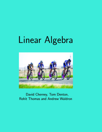
20What is Linear Algebra?linear transformation L means that L(u) can be thought of as multiplyingthe vector u by the linear operator L. For example, the linearity of L impliesthat if u, v are vectors and c, d are numbers, thenL(cu dv) cLu dLv ,which feels a lot like the regular rules of algebra for numbers. Notice though,that “uL” makes no sense here.Remark A sum of multiples of vectors cu dv is called a linear combination ofu and v.1.4So, What is a Matrix?Matrices are linear functions of a certain kind. They appear almost ubiquitously in linear algebra because– and this is the central lesson of introductorylinear algebra courses–Matrices are the result of organizing information related to linearfunctions.This idea will take some time to develop, but we provided an elementaryexample in Section 1.1. A good starting place to learn about matrices is bystudying systems of linear equations.Example 5 A room contains x bags and y boxes of fruit.20

1.4 So, What is a Matrix?21Each bag contains 2 apples and 4 bananas and each box contains 6 apples and 8bananas. There are 20 apples and 28 bananas in the room. Find x and y.The values are the numbers x and y that simultaneously make both of the followingequations true:2 x 6 y 204 x 8 y 28 .Here we have an example of a System of Linear Equations.8 It’s a collectionof equations in which variables are multiplied by constants and summed, andno variables are multiplied together: There are no powers of variables (like x2or y 5 ), non-integer or negative powers of variables (like y 1/7 or x 3 ), and noplaces where variables are multiplied together (like xy).Reading homework: problem 1Information about the fruity contents of the room can be stored two ways:(i) In terms of the number of apples and bananas.(ii) In terms of the number of bags and boxes.Intuitively, knowing the information in one form allows you to figure out theinformation in the other form. Going from (ii) to (i) is easy: If you knewthere were 3 bags and 2 boxes it would be easy to calculate the numberof apples and bananas, and doing so would have the feel of multiplication(containers times fruit per container). In the example above we are requiredto go the other direction, from (i) to (ii). This feels like the opposite ofmultiplication, i.e., division. Matrix notation will make clear what we are“multiplying” and “dividing” by.The goal of Chapter 2 is to efficiently solve systems of linear equations.Partly, this is just a matter of finding a better notation, but one that hintsat a deeper underlying mathematical structure. For that, we need rules foradding and scalar multiplying 2-vectors; 0 xcxxxx x0c: and : .ycyyy0y y0 xan unknown,yv 20 in the first line, v 28 in the second line, and L different functions in each line?We give the typical less sophisticated description in the text above.8Perhaps you can see that both lines are of the form Lu v with u 21

22What is Linear Algebra?Writing our fruity equations as an equality between 2-vectors and then usingthese rules we have: 2 x 6 y 202x 6y202620 x y .4 x 8 y 284x 8y284828Now we introduce a function which takes in 2-vectors9 and gives out 2-vectors.We denote it by an array of numbers called a matrix . 2 62 6x26The functionis defined by: x y.4 84 8y48A similar definition applies to matrices with different numbers and sizes.Example 6 (A bigger matrix) x 1 0 3 4 1034 5 0 3 4 y : x 5 y 0 z 3 w 4 . z 1 6 2 5 1625w Viewed as a machine that inputs and outputs 2-vectors, our 2 2 matrixdoes the following: 2x 6y.4x 8y xyOur fruity problem is now rather concise.Example 7 (This time in purely mathematical language): x2 6x20What vectorsatisfies ?y4 8y289 To be clear, we will use the term 2-vector to refer to stacks of two numbers such7as. If we wanted to refer to the vectors x2 1 and x3 1 (recall that polynomials11are vectors) we would say “consider the two vectors x3 1 and x2 1”. We apologizethrough giggles for the possibility of the phrase “two 2-vectors.”22

1.4 So, What is a Matrix?23This is of the same Lv w form as our opening examples. The matrixencodes fruit per container. The equation is roughly fruit per containertimes number of containers equals fruit. To solve for number of containerswe want to somehow “divide” by the matrix.Another way to think about the above example is to remember the rulefor multiplying a matrix times a vector. If you have forgotten this, you canactually guess a good rule by making sure the matrix equation is the sameas the system of linear equations. This would require that 2 6x2x 6y: 4 8y4x 8yIndeed this is an example of the general rule that you have probably seenbefore p qxpx qypq: x y.r syrx syrsNotice, that the second way of writing the output on the right hand side ofthis equation is very useful because it tells us what all possible outputs amatrix times a vector look like – they are just sums of the columns of thematrix multiplied by scalars. The set of all possible outputs of a matrixtimes a vector is called the column space (it is also the image of the linearfunction defined by the matrix).Reading homework: problem 2Multiplication by a matrix is an example of a Linear Function, because ittakes one vector and turns it into another in a “linear” way. Of course, wecan have much larger matrices if our system has more variables.Matrices in Space!Thus matrices can be viewed as linear functions. The statement of this forthe matrix in our fruity example is as follows. 2 6x2 6x1.λ λand4 8y4 8y23

24What is Linear Algebra? 2.2 64 8 0 0 2 6x2 6xxx. y0y04 8y4 8yThese equalities can be verified using the rules we introduced so far. 2 6Example 8 Verify thatis a linear operator.4 8The matrix-function is homogeneous if the expressions on the left hand side and righthand side of the first equation are indeed equal. 2 6a2 6λa26λ λa λb4 8b4 8λb48 2λa6bc2λa 6λb 4λa8bc4λa 8λbwhile λ2 64 8 6b2a62a λ b c a8b4a84b 2λa 6λb2a 6b. λ4λa 8λb4a 8bThe underlined expressions are identical, so the matrix is homogeneous.The matrix-function is additive if the left and right side of the second equation areindeed equal. 2 64 8 62a c2 6ca (b d) (a c) 84b d4 8db 2(a c)6(b d)2a 2c 6b 6d 4(a c)8(b d)4a 4c 8b 8dwhich we need to compare to 2 6a2 6c2626 a b c d4 8b4 8d4848 2a6b2c6d2a 2c 6b 6d .4a8b4c8d4a 4c 8b 8dThus multiplication by a matrix is additive and homogeneous, and so it is, by definition,linear.24

1.4 So, What is a Matrix?25We have come full circle; matrices are just examples of the kinds of linearoperators that appear in algebra problems like those in section 1.3. Anyequation of the form M v w with M a matrix, and v, w n-vectors is calleda matrix equation. Chapter 2 is about efficiently solving systems of line

algebra is, in general, the study of those structures. Namely Linear algebra is the study of vectors and linear functions. In broad terms, vectors are things you can add and linear functions are functions of vectors that respect vector addition. The goal of this text is to teach you to organize information about vector spaces in a way that makes