Transcription
THESISARE WILD AND SCENIC RIVERS REALLY “FREE-FLOWING”?Submitted byKathryn Rosalie WilliDepartment of Ecosystem Science and SustainabilityIn partial fulfillment of the requirementsFor the Degree of Master of ScienceColorado State UniversityFort Collins, ColoradoSpring 2021Master’s Committee:Advisor: Stephanie K. KampfCo-Advisor: Matt R. V. RossLynn Badia
Copyright by Kathryn Rosalie Willi 2021All Rights Reserved
ABSTRACTARE WILD AND SCENIC RIVERS REALLY “FREE-FLOWING”?This study quantified the “free-flowing” character of wild and scenic river watersheds byfirst developing linear regression models to predict the “natural condition” of a river’smagnitude, timing, frequency, and variability of flows. We compared these estimates of“natural” flow to the observed values for stream gages within wild and scenic river watershedsand found that nearly half (45.1%) had at least one altered flow metric. This was significantlylower (p 0.05) than the fraction of altered gages outside wild and scenic river watersheds, andsupported our other conclusion that wild and scenic rivers are associated with protected areas.On the other hand, wild and scenic river watersheds had a significantly higher (p 0.05) fractionof gages with dam storage densities 100 megaliters·km-2 than gages outside wild and scenicriver watersheds. Because the Wild and Scenic Rivers Act was designed as a complement to damdevelopment, many wild and scenic rivers are designated in direct response to the threat of damconstruction, or to counterbalance special rivers that have already been dammed. We posit thatthis biases wild and scenic river designations towards locations where dam development iscommon. Our study’s findings expose a paradox in how a wild and scenic river designation canfully “protect and enhance” a river’s free-flowing character. True protection of these specialresources does not stop at designation, and requires additional support from managing agenciesand stewardship groups to make improvements to their watersheds.ii
ACKNOWLEDGEMENTSI would first like to sincerely thank my advisors, Stephanie Kampf and Matt Ross. Iwould not have been able to make it through this journey without their insight, guidance, andextreme kindness. I am also grateful to Abby Eurich, who was instrumental in helping me firstnavigate the world of linear regression modelling in R. Lynn Badia’s literature recommendationswere also critical in the completion of this work, particularly in helping give context to myfindings. I would also like to take this opportunity to thank Jennifer Back with the National ParkService, who has been a mentor to me throughout this wild (and scenic!) experience and whomade this research possible.iii
TABLE OF CONTENTSABSTRACT. iiACKNOWLEDGEMENTS . iii1. INTRODUCTION . 12. BACKGROUND . 33. METHODS . 93.1 Calculating “Free-Flow” Metrics . 103.2 Selecting Reference Watersheds . 123.3 Grouping Watersheds of the Contiguous US . 133.4 Developing the Models . 153.5 Predicting and Assessing “Natural” Flow. 184. RESULTS . 204.1 Seasonal Distribution of Flows . 254.2 High and Low Flows . 284.3 Variability, Frequency, and Duration of Flows . 295. DISCUSSION . 315.1 Comparison to Other Stream Gage Assessments. 315.2 Wild and Scenic River Modifications and the “Free-Flowing” Paradox . 325.3 Partnership Wild and Scenic Rivers . . 365. 4 Caveats to our Evaluation . 376. CONCLUSION . 40BIBLIOGRAPHY . 42APPENDIX . 50iv
1. INTRODUCTIONThe National Wild and Scenic River System is a collection of rivers that are supposed toreceive the highest level of river protection in the United States (US). From the far reaches ofAlaska to the jungles of Puerto Rico, the National System currently “protects” over 500 streamsfor their free-flowing character, their water quality, and the “outstandingly remarkable values”that make them unique at a regional or national scale (16 U.S. Code 1271-1278). Safeguardedunder the National Wild and Scenic Rivers Act of 1968, this collection of rivers shared betweenthe US Forest Service, the US Fish and Wildlife Service, the Bureau of Land Management, andthe National Park Service is seen internationally as a model method for river conservation at atime when river protection has become a global priority (Palmer, 2017; IUCN, 2020).Under the Wild and Scenic Rivers Act, river managing agencies must “protect andenhance” a wild and scenic river’s free-flowing character, which the Act defines as “existing orflowing in natural condition without impoundment, diversion, straightening, rip-rapping, orother modification of the waterway” (16 U.S. Code 1271-1278). To maintain a wild and scenicriver’s free-flowing status, the Act prohibits federally funded water resource projects “on ordirectly affecting” the river, and projects up or downstream of the designated corridor that“invade the area or unreasonably diminish” the values that had it designated. Although thedesignated corridor is protected from federally assisted water resource projects, a wild and scenicriver designation does not fundamentally protect its entire watershed. Upstream reaches, andeven designated reaches, may still have impoundments, diversions, or other circumstances thathave the potential to modify the “natural condition” of wild and scenic rivers by altering themagnitude, timing, and variability of their flow regimes (Poff et al., 1997). Therefore, the goal of1
this study is to assess the extent to which wild and scenic river corridors and their contributingwatersheds are truly “free-flowing”.2
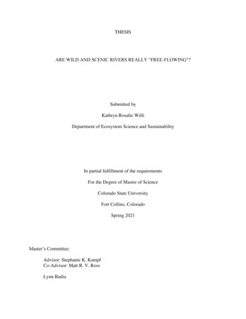
2. BACKGROUNDCurrently there are 230 designated wild and scenic rivers in the system1 (Figure 1),though many designations incorporate more than one river. For example, the Smith Wild andScenic River in California embodies the Smith River as well as 62 of its tributaries, while theWekiva Wild and Scenic River in Florida includes the Wekiva River as well as Rock SpringsRun and Blackwater Creek. Consequently, the system’s true number of protected streams liescloser to 520 (updated from Palmer, 2017). The National Wild and Scenic River Systemcaptures many different types of rivers: from the historic Delaware River in the mid-Atlantic,to the desert oasis of Surprise Canyon Creek in Death Valley, to the mountainous headwatersof the Snake River in Wyoming. Spatially, there are large concentrations of wild and scenicrivers in Alaska, the Pacific Northwest, and the Great Lakes regions, though 40 states andPuerto Rico have at least one wild and scenic river. The lengths of designated reaches rangefrom under one kilometer to over 600 kilometers. Watershed sizes also vary substantially; thewild and scenic river with the largest contributing area is the Missouri Wild and Scenic Riverin South Dakota and Nebraska (785,119 km2), while the smallest is Spring Creek in Oregon(2.1 km2). Regardless of these differences, all wild and scenic rivers are protected for thevalues that got them designated: their water quality, their outstandingly remarkable rivervalues, and their free-flowing condition.1The official number of designated wild and scenic rivers is 226. However, the Delaware Wild and Scenic River,the Rio Grande Wild and Scenic River, and the Klamath Wild and Scenic River have been split into separate wildand scenic rivers for this analysis based on how the Interagency Wild and Scenic River Coordinating Council treatsthem.3
Figure 1. Histograms depicting the distribution of wild and scenic river (WSR) lengths and watershedsizes, and a map of the WSR System and its contributing watersheds. The River Styx in Oregon,WSRs in Alaska and Puerto Rico, and WSRs whose watersheds are 100,000 km2 were excludedfrom our analysis.Because streamflow is a dominant driver of a river’s water quality, ecological diversity,and channel geomorphology, it is often considered the “master variable” of river function (Poweret al., 1995; Poff et al., 2010). Therefore, the “natural condition” of streamflow is not only acritical component of the free-flowing requirements of the Wild and Scenic Rivers Act, it is alsointimately linked to a wild and scenic river’s water quality and the status of many outstandingly4
remarkable values. The fluctuations in streamflow and their timing have major implications onthe concentrations of chemical constituents in the stream, how they are transported, and how theyare transformed (Kagawa 1992; Tu, 2009; Wei et al., 2009; Fantin-Cruz et al., 2016). Manyoutstandingly remarkable values also directly rely on the magnitude, timing, and range of naturalflows. For example, the Virgin Wild and Scenic River in Utah has been designated in part for itsexceptional ecological value; the rare plant communities and cottonwood galleries that existthere depend on the river’s seasonal flooding (US Department of Interior, 2013b). The range andvariability of streamflow, coupled with changing sediment loads, are often critical in supportinga rich and diverse community of native plants and animals (Junk, Bayley, and Sparks, 1989; Poffet al., 1997; Hart and Finelli, 1999). Another example is the Snake River Headwaters Wild andScenic River, whose geologic values rely on specific flow magnitudes for the uniquegeomorphologic features found there (US Department of Interior, 2013a). Dynamic flows canalso support a wide range of recreation opportunities (Brown, Taylor, and Shelby, 1992). Forinstance, the Bluestone Wild and Scenic River’s recreational values rely on high flows forpaddling activities, and lower flows for safe wading, fishing, and swimming (Nadeau et al.,2018).Yet, there is limited information regarding the extent to which streams have beenmodified within wild and scenic river watersheds. Some assessments have been conducted forindividual wild and scenic rivers (e.g., Narvaez and Homsey, 2016; OARS for the Assabet,Sudbury, and Concord Rivers, 2019; Elmore et al., 2020), but there has been no comprehensiveeffort to assess the flow conditions of the entire system. At a broader level of investigation, Grillet al. (2019) found that 63% of the world's large rivers are no longer free-flowing, whileHarrison-Atlas et al. (2017) found that 49% of all river miles in the Western US are5
hydrologically altered. Moreover, a recent report by the US Geological Survey (USGS) foundthat 80% of the USGS stream gages they assessed had altered flow (Eng et al., 2019).Extrapolating from Eng et al. (2019)’s findings, Carlisle et al. (2019) posits that over one third ofall streams in the contiguous US have human-modified streamflow. An analysis of wild andscenic river water quality also revealed that states have identified multiple wild and scenic riversas having impaired streamflow under the Clean Water Act (Willi and Back, 2018). Collectivelythese findings suggest that hydrologic alteration may be widespread in the system, despite wildand scenic river legal protections.Though not specific to wild and scenic rivers, several frameworks have been developedto address questions surrounding the hydrologic character of streams and their watersheds.Thornbrugh et al. (2018) developed a watershed assessment framework that uses nationallyavailable datasets on land use, dam density, fertilizer application rates, and other watershedcharacteristics to assess the likely extent of hydrologic modification. Along those lines, the USEnvironmental Protection Agency (EPA) developed the Watershed Index Online tool that allowsusers to develop watershed condition indices based on a similar set of nationally availabledatasets for any HUC-12 watershed in the conterminous US (EPA, 2017). Because thesewatershed assessment strategies are intended to be used for all streams of the US with aconsistent approach, they do not incorporate actual streamflow observations into theirframeworks.An example of a localized approach for measuring a stream’s hydrologic character is theNature Conservancy (2009)’s Indicators of Hydrologic Alteration tool, where users input dailystreamflow data to calculate ecologically relevant flow metrics through time. With informationrelated to changes made to a stream’s watershed, such as dam development or a change in land6
use, the tool calculates the mean or variance of the flow statistics across the time period beforeand after the disturbance. Comparative statistical analysis between these periods then allows theuser to determine whether the disturbance significantly changed streamflow. Because this toolrequires knowledge of when changes in the watershed occurred, it is most useful for answeringriver-specific questions related to streamflow.Another common way of assessing hydrologic character is to develop models that predictnatural streamflow across individual states or regions, and compare the modeled values toobserved streamflow (e.g., Sanborn and Bledsoe, 2006; Ries et al., 2017; Eurich, 2020). Onesuch application has been implemented as part of the National Hydrography Dataset, whichprovides estimates of mean monthly and annual streamflow across all stream features in itsdataset (McKay et al., 2012; Moore et al., 2019). These streamflow metrics are first estimated byusing a water balance model (McCabe and Wolock, 2011), thereby providing an estimate ofnatural streamflow. These natural estimates can then be adjusted using a regression equation tomatch nearby stream gage records, providing a value more consistent with observed streamflowpatterns.In France, Snelder et al. (2009) developed boosted regression trees that grouped streamsby their flow regimes to predict natural flow metrics related to the frequency, magnitude, timing,and variability of daily flows. Using unmodified streamflow stations to train the models, theyfound watershed characteristics such as slope, watershed area, temperature, and soil permeabilitywere effective predictor variables for identifying a stream’s flow regime.Similarly, Eng et al. (2019) developed random forest models predicting naturalstreamflow metrics across the contiguous US that could be compared to observed streamflow,landscape characteristics including urbanization, dam density and agriculture, and climate7
variability. Their assessment used stream gages in the GAGES-II database (Falcone, 2011),which includes both small headwater watersheds as well as large river basins up to 49,600 km2.They found that 80% of the 3,355 gages analyzed were altered to some degree, with landscapecharacteristics being a more dominant driver of changes in streamflow compared to climatevariability. Here, we build on the methods of Eng et al. (2019) by developing regional regressionmodels that capture the “natural condition” of the flow regime for USGS stream gages withinand outside wild and scenic river watersheds.8
3. METHODSThis analysis focuses on wild and scenic river watersheds within the contiguous US;including watersheds within Alaska and Puerto Rico would have required datasets that are not asreadily available and nationally consistent. For example, there are only four USGS stream gagesin the entire wild and scenic river system of Alaska, which spans a collective area of 131,618km2. We also excluded the Snake Wild and Scenic River in Oregon and Idaho, the Missouri Wildand Scenic River in Montana, South Dakota, and Nebraska, the Green Wild and Scenic River inUtah, and the Rio Grande Wild and Scenic River in Texas from our study because theirwatersheds are so large ( 100,000 km2) that this type of analysis would not be appropriate.Furthermore, we already know these large wild and scenic river watersheds are altered due totheir national importance for irrigation, commerce, and hydropower (Reisner, 1993). The RiverStyx in Oregon was also excluded because both the designated reach and its watershed arealmost exclusively underground. This reduces our analysis to 196 of the 230 designated wild andscenic rivers (Figure 1).To characterize the “free-flowing” status of wild and scenic river watersheds, weevaluated whether their flow regimes had been substantially altered from their “naturalcondition”. We define “natural condition” as an unmodified river’s mean annual flow, high andlow flow magnitude (Q99, Q1) and variability (CVhigh, CVlow), frequency (Fhigh, Flow) andduration (Dhigh, Dlow) of high and low flow pulses, and the seasonal distribution (S) of dailyflows. To quantify these components of the flow regime, we developed linear regression modelsusing reference-quality USGS stream gages to predict the “natural condition” of streams withinwild and scenic river watersheds.9
3.1 Calculating “Free-Flow” MetricsDaily streamflow for each stream gage used in our study was downloaded from theUSGS National Water Information System using the ‘dataRetrieval’ package in R (De Cicco etal., 2018; USGS, 2020). All data was then area-normalized to mm·day-1. To best representcurrent flow conditions, we only analyzed streamflow data from the period of 1980 to 2019.1980 was selected as the cutoff because the development of most major water projects that couldsignificantly modify flow (e.g., large reservoirs and large-scale diversions) occurred before then,and the major patterns in land and water management have not changed significantly since then(Eng et al., 2019).The one-day low and high magnitudes (Q1 and Q99, respectively) were calculated as the1st and 99th percentile non-exceedance daily flow from each stream gage’s chosen period ofrecord (i.e., 1980-2019). Annual high and low flow variability (CVhigh and CVlow, respectively)were calculated by identifying each water year’s maximum and minimum daily flow thendetermining their coefficient of variation:CVlow sdlow / meanlowCVhigh sdhigh / meanhighwhere sdx represents the annual standard deviation of the minimum or maximum flows andmeanx represents the annual mean low and high flow. High and low flow frequency (Fhigh andFlow, respectively) were calculated by computing each year’s total number of high or low pulses,then averaging the number of high or low pulses across all years. A high pulse was defined as aset of consecutive days ( 2 days) in which the flow was at or above the 90th percentile flow, anda low pulse was defined as a set of consecutive days in which the flow was at or below the 10thpercentile non-exceedance daily flow. High flow duration (Dhigh) was calculated as the mean10
number of days per water year that the flow was at or above the 90th percentile non-exceedancedaily flow. Low flow duration (Dlow) was calculated as the mean number of days per water yearthat the flow was at or below the 10th percentile flow. Seasonality was calculated as the fractionof the total annual flow (in mm) that falls within a given season, for each year. Those fractionswere then averaged across each year to get the mean fraction of flow for each season. See Table1 for a list of all flow metrics analyzed in our study.Table 1. Flow metrics used to represent a stream’s “natural condition”. Asterisks represent flow metricsused in Eng et al. (2019).Flow MetricDescriptionQmeanMean annual flowAutumnMean annual fraction of total flow in September, October, and NovemberWinter FlowsMean annual fraction of total flow in December, January, and FebruarySpring FlowsMean annual fraction of total flow in March, April, and MaySummerMean annual fraction of flow in June, July, AugustQ99*99th percentile non-exceedance flowQ1*1st percentile non-exceedance flowCVhigh*Coefficient of variation of annual maximum daily flowsCVlow*Coefficient of variation of annual minimum daily flowsFhigh*Mean number of annual flow pulses greater than the 90th percentile non-exceedance flowFlow*Mean number of annual flow pulses less than the 10th percentile non-exceedance flowDhigh*Mean annual duration of flow pulses greater than the 90th percentile non-exceedance flowDlow*Mean annual duration of flow pulses less than the 10th percentile non-exceedance flow11
3.2 Selecting Reference WatershedsModels for predicting natural streamflow were developed using a subset of stream gagesidentified as being of reference quality by Falcone (2011). From Falcone (2011), we selectedonly stream gages whose watersheds were smaller than 1,500 km2 to minimize the potential forwithin-basin variability in streamflow generation (Hammond and Kampf, 2020; Eurich, 2020).Stream gages whose watersheds crossed international boundaries were removed from theanalysis due to limitations in the spatial extent of most datasets in this study. Referencewatersheds were further screened for characteristics with known impacts to the natural flowregime including transbasin diversions, dams, major wastewater treatment facilities, urban landcover, and cropland.To identify transbasin diversions we used the High-Resolution National HydrographyDataset (Moore et al., 2019) to detect ditches, canals, and pipelines that crossed watershedboundaries. We also identified watersheds with dam storage densities of over 100 megaliters·km-2, which Eng et al. (2019) used as the threshold at which a watershed is categorized as damaltered. Using a similar methodology to Harrison-Atlas et al. (2017), we used the NationalInventory of Dams’ normal storage variable (USACE, 2019) to compute dam storage densities.Major wastewater treatment facilities that discharge 1 million gallons·day-1 were identifiedusing the EPA’s Wastewater Treatment Plants geodatabase (EPA, 2020). Land covercharacteristics including percent cropland and imperviousness were computed from the 2011National Landcover Dataset (Wickham et al., 2014). Urban watersheds were defined aswatersheds with 5% or greater mean impervious land cover as suggested by Bhaskar and Welty(2012). We considered a watershed with 2.5% cropland or greater to be agricultural. This cutoffwas based on visual inspection of the mean annual flow of a stream gage’s watershed against the12
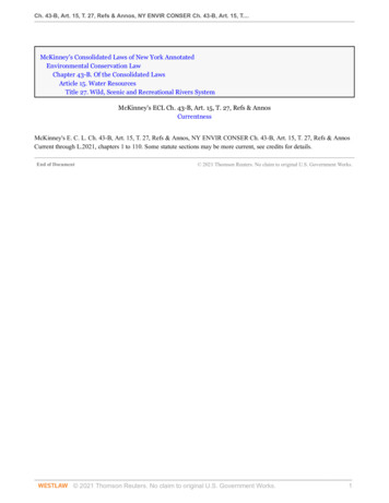
mean aridity index of the watershed; at a given aridity index, watersheds with over 2.5%cropland tend to have lower mean annual streamflow than those with less than 2.5% cropland(Figure A1 in the Appendix).The final dataset included watersheds with no transbasin diversions, dam storagedensities under 100 megaliters۰km-2, no major wastewater treatment facilities, less than 5%mean urban impervious cover, and less than 2.5% of crop land cover. Beyond these watershedcharacteristic requirements, only stream gages with at least 20 years of complete data (i.e., a100% complete period of record for a water year) between the 1980-2019 period were included,leaving a dataset of 642 reference gages.3.3 Grouping Watersheds of the Contiguous USBecause of the diversity of climate, soil, and land cover conditions for the contiguous US,strong models could not be developed using all of the gages together. Instead, we chose to dividethem into regions, each analyzed individually. However, our strict criteria for selecting referencewatersheds created a set of stream gages that were not evenly distributed in space, leaving largeswaths of the US unrepresented, particularly the Midwest (Figure 2). If we based regionalizationon the National Rivers and Stream Assessment ecoregions (EPA, 2016), for instance, therewould be only one viable stream gage in the Temperate Plains region, one viable stream gage inthe Northern Plains region, and only 11 viable stream gages in the Upper Midwest. Therefore,we developed a grouping mechanism that relied on other factors that are linked to streamflowgeneration. We grouped watersheds together based on their mean aridity index, soil sand content,and geographic location. Each watershed was identified as having a mean aridity index above orbelow one, having a mean soil content above or below 53% sand, and being either predominantlyeast or west of the 100th meridian.13
Figure 2. Map showing model regions, and the stream gages associated with them. We divided thecontiguous US into eight regions: east, aridity index 1 (surplus, S), not sandy (E-S-NS, n 146); east,aridity index 1, sandy (E-S-S, n 53); east, aridity index 1 (deficit, D), not sandy (E-D-NS, n 97);east, aridity index 1, sandy (E-D-S, n 29); west, aridity index 1, not sandy (W-S-NS, n 74); west,aridity index 1, sandy (W-S-S, n 58); west, aridity index 1, not sandy (W-D-NS, n 111); and west,aridity index 1, sandy (W-D-S, n 74).The mean aridity index of a watershed, which is calculated as the mean ratio betweenprecipitation and potential evapotranspiration, was used to define sub-regions because it broadlycaptures a given watershed’s relationship to water; if a watershed’s mean aridity index fallsbelow one, it indicates that the watershed’s ability to lose water to the atmosphere is greater thanthe amount of precipitation it receives (i.e., water deficit, D). Inversely, if a watershed’s meanaridity index is greater than one, the watershed generally receives more water than it can lose tothe atmosphere (i.e., water surplus, S).The sand content of soil was used because locations with sandy soils tend to behavedifferently than non-sandy soils when assessing regional patterns of streamflow; sandy soilstypically lead to faster rates of infiltration and higher hydraulic conductivities (Twarakavi,14
Šimůnek, and Schaap, 2010). The chosen threshold of 53% sand was selected based on theUSDA Natural Resource Conservation Service’s soil texture triangle; all soil textures areconsidered “sandy” past 53% sand (Vanlear, 2019). Moreover, this closely captures Twarakavi,Šimůnek, and Schaap (2010)’s sand-dominated hydraulic classification groups. Lastly, the 100thmeridian was selected as a geographic grouping mechanism because it approximates the point atwhich the elevation begins to rise on its way towards the Rocky Mountains, and levels ofprecipitation tend to change (Gesch et al., 2002). Ultimately, the combination of theseaggregating mechanisms resulted in a total of eight unique watershed groups (Figure 2): east,aridity index 1 (water surplus, S), not sandy (E-S-NS, n 146); east, aridity index 1, sandy (ES-S, n 53); east, aridity index 1 (water deficit, D), not sandy (E-D-NS, n 97); east, aridityindex 1, sandy (E-D-S, n 29); west, aridity index 1, not sandy (W-S-NS, n 74); west, aridityindex 1, sandy (W-S-S, n 58); west, aridity index 1, not sandy (W-D-NS, n 111); and west,aridity index 1, sandy (W-D-S, n 74). For each of the eight watershed groups, 13 linearmodels were developed to predict each of the flow metrics of interest, resulting in 104 uniquemodels.3.4 Developing the ModelsWatershed boundaries for the stream gages used in model development were obtainedfrom the GAGES-II database (Falcone, 2011). Using the geospatial software ArcGIS (ESRI,2017), 32 variables related to climate, topography, soil properties, geology, and land cover werecomputed for each watershed (see Table 2). These variables were chosen as potential predictorsbecause they have been used in previous models that predict streamflow statistics, and/or have anestablished relationship to streamflow generation (Hortness and Berenbrock, 2001; Snelder et al.,2009; Carlisle et al., 2010; Gotvald, 2017; Eurich, 2020).15
Table 2. Watershed and stream attributes used as predictor variables in the regression models.VariableSourceStream Gage Latitude (NAD83)NWIS (USGS, 2020)Stream Gage Longitude (NAD83)NWIS (USGS, 2020)Stream Gage Elevation (m)National Elevation Dataset (NED; Gesch et al., 2002)2Watershed Area (km )NED (Gesch et al., 2002)Mean Watershed Elevation (m)NED (Gesch et al., 2002)Median Watershed Elevation (m)NED (Gesch et al., 2002)Mean Watershed Slope (%)NED (Gesch et al., 2002)Percent Watershed with Slope over 30 (%)NED (Gesch et al., 2002)Dominant AspectNED (Gesch et al., 2002)Mean Base-Flow IndexUSGS (Wolock, 2003)Mean Erodibility FactorSSURGO (NRCS USDA, 2019)Mean Soil Organic Matter (%)SSURGO (NRCS USDA, 2019)Mean Soil Permeability (mm)SSURGO (NRCS USDA, 2019)Mean Clay (%)SSURGO (NRCS USDA, 2019)M
flowing in natural condition without impoundment, diversion, straightening, rip-rapping, or other modification of the waterway" (16 U.S. Code 1271-1278). To maintain a wild and scenic river's free-flowing status, the Act prohibits federally funded water resource projects "on or


![INDEX [randycherry ]](/img/21/x-20-20tv-20fakebook-20-20hal-20leonard.jpg)