Transcription
HindawiApplied Computational Intelligence and So ComputingVolume 2022, Article ID 1562942, 11 pageshttps://doi.org/10.1155/2022/1562942Research ArticleHybrid Machine Learning Model for Electricity ConsumptionPrediction Using Random Forest and Artificial Neural NetworksWitwisit Kesornsit1 and Yaowarat Sirisathitkul21Government Data Solution Division, Department of Data Solution,Digital Government Development Agency (Public Organization), Bangkok, Thailand2Department of Computer Engineering and Electronics, School of Engineering and Technology, Walailak University,Nakhon Si Thammarat, ThailandCorrespondence should be addressed to Yaowarat Sirisathitkul; kinsywu@gmail.comReceived 24 October 2021; Accepted 9 April 2022; Published 21 April 2022Academic Editor: Cheng-Jian LinCopyright 2022 Witwisit Kesornsit and Yaowarat Sirisathitkul. This is an open access article distributed under the CreativeCommons Attribution License, which permits unrestricted use, distribution, and reproduction in any medium, provided theoriginal work is properly cited.Predicting electricity consumption is notably essential to provide a better management decision and company strategy. This studypresents a hybrid machine learning model by integrating dimensionality reduction and feature selection algorithms with abackpropagation neural network (BPNN) to predict electricity consumption in Thailand. The predictive models are developed andtested using an actual dataset with related predictor variables from public sources. An open geospatial data gathered from a realservice as well as geographical, climatic, industrial, household information are used to train, evaluate, and validate these models.Machine learning methods such as principal component analysis (PCA), stepwise regression (SWR), and random forest (RF) areused to determine the significant predictor variables. The predictive models are constructed using the BPNN with all availablevariables as baseline for comparison and selected variables from dimensionality reduction and feature selection methods. Alongwith creating a predictive model, the most related predictors of energy consumption are also selected. From the comparison, thehybrid model of RF with BPNN consistently outperforms the other models. Thus, the proposed hybrid machine learning modelpresented from this study can predict electricity consumption for planning and managing the energy demand.1. IntroductionDue to the pandemic crisis in 2020, total energy demandduring 2020–2030 is likely to be higher than the International Energy Agency (IEA) forecast. Electricity consumption has become one of the critical issues in most countries.Therefore, the accurate prediction of electricity consumptionhas an essential role in achieving efficient energy utilization.Assessment of the electricity consumption in advance willimprove operation strategies and management of energystorage system and planning activities for future powerplants [1, 2]. One of the largest electricity consumers is thebusiness sector. Generally, socioeconomic and environmental factors contribute to electricity consumption. Socioeconomic factors include industrial and householdinformation, while environmental factors includegeographical and climatic information. Determining thesignificant relation of different factors related to electricityconsumption could provide guidelines for electricity authority management to carry out the planning and strategiesin an efficient manner.Over the past several decades, many statistical andcomputational intelligence methods have been implementedin the fields of prediction. Previous studies are mainlylimited to a small dataset of independent variables based ontime-series forecasting, regression analysis, and clusteringmethods [3, 4]. The statistical methods have some restrictions on the linearity, normality, and independence ofvariables [5]. Computational intelligence methods, such asartificial intelligence algorithms, have been primarilyimplemented in prediction [6]. Recent research shows thatthe super computing power is more efficient and effective in
2handling and analyzing huge volumes of data. The machinelearning algorithms, a subset of artificial intelligence, exhibitsuperior performance in handling large numbers of data [7].The majority of research in electricity consumptionmodeling uses various machine learning methods, in particular artificial neural network (ANN), decision tree, andclustering. Platon et al. [1] performed research on ANNconcerning the hourly prediction of electricity consumption.Walker et al. [8] predicted the energy consumption of thebuilding using random forest (RF) and ANN. Pérez-Chacónet al. [9] proposed a methodology for finding patterns ofelectricity consumption using the k-means. Shi et al. [10]employed echo state network in the prediction of buildingenergy demand. Furthermore, the literature review onmachine learning algorithms in energy research has beenproposed by Mohandes et al. [11] and Lu et al. [12].Moreover, the current research of predicting the futureelectricity demand related to hybrid models combining different two or more machine learning algorithms was reviewedand analyzed by Deb et al. [13] and Mamun et al. [14]. Thehybrid models show excellent results because individual algorithms have different advantages. Zekić-Sušac et al. [4]integrated the variable selection with ANN in developing apredictive model for the energy cost of public buildings inCroatia. Zekić-Sušac et al. [15] integrated clustering and ANNto improve the accuracy of modeling energy efficiency.Muralitharan et al. [16] proposed a convolutional neuralnetwork based optimization approach for predicting thefuture energy demand. Pérez-Chacón et al. [17] used a bigdata time-series and experimental method with decision tree,gradient boosting machine (GBM), pattern sequence-basedforecasting, ARIMA, and ANN to forecast the electricitydemand. Zekić-Sušac et al. [18] used variable reductionprocedures with RPart regression tree, RF, and deep neuralnetworks to construct a predictive model for the energydemand of public buildings in Croatia. Basurto et al. [19]employed a hybrid intelligent system based on ANN andclustering algorithm to predict the solar energy in Spain.Therefore, it is appropriate to exploit machine learning algorithms in electricity consumption prediction.This study has demonstrated the prediction of electricityconsumption. The proposed procedure has several phases:data collection and data preprocessing, dimensionality reduction and feature selection, and prediction. In the datacollection and data preprocessing phase, the data is collectedfrom publicly available sources and processed to handle themissing values and outliers. In the dimensionality reductionand feature selection phase, the techniques includingprincipal component analysis (PCA), stepwise regression(SWR), and RF are applied. The prediction phase isimplemented by using the backpropagation neural networks(BPNN) algorithm. The selected important predictor variables from PCA, SWR, and RF have been used as the inputsfor the BPNN algorithm to predict the electricity consumption. Besides creating a predictive model, the subset ofrelevant variables is also selected and compared. Six metricsevaluate the effectiveness of the predictive models. Themodel with the highest accuracy in the test evaluation hasbeen selected.Applied Computational Intelligence and Soft ComputingThe other sections of this paper are as follows. Section 2introduces the machine learning algorithms employed inthis study and exploration of the relevant literature. Section3 outlines the architecture of the proposed predictivemodels, experimental dataset, and the evaluation method.Section 4 describes the experimental outcome and somestatistical results. Finally, Section 5 gives the paperachievement as well as the conclusions and future works.2. Literature ReviewMachine learning is an algorithm to construct empiricalmodels from the dataset and is categorized as data-drivenmodeling requiring a sufficient quantity of historical data topredict future demand reliably [8]. Machine learning algorithms extract essential information presented in largeamounts of the recorded data, thereby achieving betterperformance and accuracy [7, 20]. Systematic literaturereviews of artificial intelligence and machine learning algorithms are provided by Duan et al. [21], Borges et al. [22],and Dwivedi et al. [23]. It is accepted that these techniquesbring a significant impact and new research frameworks inindustries such as finance, medicine, manufacturing, andvarious government, public sector, and business domains.For example, the machine learning methodology isemployed in the prediction of crime [24], future price ofagricultural products [25], natural gas consumption [26],commercial banks performance [27], landslide displacement[28], and seawater evaporation [29]. As may be seen, prediction algorithms have been extensively investigated inseveral sectors.Constructing the predictive models by employing a lot ofvariables is not straightforward in practice. All these variables might not be completely collected in a real-worldsituation and result in a more complex model. The prominence of dimensionality reduction and feature selection ofmodeling variables have been broadly revealed in [30]. ThePCA is the most common feature extraction method toreduce the dimensionality of large dataset into a smalldataset that retains most of the information [31]. The PCAuses the eigenvalue and eigenvector for projecting the highdimensional dataset on to a lower-dimensional space. Itconverts a set of correlated variables into a set of principalcomponents. Only the principal components that can sustain the most original variance will be extracted [32, 33].Dimensionality reduction with the PCA is applied in manydomains such as electricity consumption [1], finance [31],engineering [34], and agriculture [35, 36]. The disadvantageof PCA is that the predictor variables become less interpretable and have no corresponding physical meaning andthis makes it more challenging to determine the predictorvariables that are important in the predictive model [35, 37].Feature selection is a process to select the features thatcontain the most useful information while discarding redundant features that contain little to no information. Thewrapper feature selection algorithm such as SWR and RF is amethod that depends on the accuracy of the subsequentfeature selection criterion. The SWR is a statistical method offitting regression models and has the advantage of evading
Applied Computational Intelligence and Soft Computingcollinearity [38]. It defines appropriate variable subsets andevaluates variables priorities [39]. Selection of predictorvariables is performed automatically by assessing the relativeimportance of the variables based on prespecified criteriasuch as the F-test, the t-test, the adjusted R2, and the Akaikeinformation criterion (AIC).The RF is a supervised machine learning algorithm that iseffective and efficient for both classification and prediction.It is based on a decision tree algorithm and classified as abagging ensemble learning method [24, 40]. The RFstructure is composed of multiple decision trees, and theneach RF tree runs in a parallel manner to each other. Duringthe variable randomization in each iteration, a variableimportance index and the Gini index can be given [41]. Thefinal value is evaluated by aggregating the results from allleaves of each tree [35, 42]. The RF is also one of the bestalgorithms for estimating the importance of variables and isapplied in various fields [20, 43–45]. Furthermore, the RF isan excellent prediction algorithm and has the advantages ofits generalization and a good balance of error [11, 46, 47].Some analysts employed both SWR and RF to select theinput variables or analyze the importance of variables indomains such as the electronic industry [5], geographicalpoverty [45], reservoir characterisation [48], and soil carbon[49]. They stated that RF is better than SWR in identifyingnonlinear relationships between variables.The ANN is classified as a supervised learning methodand also deployed in the comparison of prediction performance with other machine learning techniques [50–55].Among the ANN, BPNN is one of the most widely usedtechnique to optimize the feedforward neural network. Thebackpropagation algorithm is a broadly used technique anda standard method for training the weights in a multilayerfeedforward neural network through a chain rule method[56]. The weights of a neural net are appropriately adjustedbased on the loss in the previous iteration. Therefore, thisresults in a lower error rate, making the model more reliableby enhancing a generalization. Researchers have appliedBPNN in many classifications and predictions. As an example, BPNN is employed in agricultural product sales [57],crude oil future price [58], and hybrid cement [59] and alsodeployed in the comparison of prediction performance withother machine learning techniques [50–52].3. Materials and MethodsThe outline of the proposed framework is shown in Figure 1.The hybrid predictive model comprises three stages conducting in sequence. The first stage explores the exploratorydata analysis. The second stage uses the PCA, SWR, and RFmethods to select suitable predictor variables. The third stageis to establish the predictive model by constructing theBPNN. The developed models are trained with 10-fold crossvalidation and evaluated. All models have been implementedand tested on intel Core i7-8550U, CPU @1.80 GHz,1.99 GHz running, 64 bit Windows 10 operating system with8 GB RAM. The Scikit-learn machine learning package forthe Python programming language is used to implement themodels with Python version 3.9.4. Many algorithms 3StartData collection and Data preprocessingCorrelation and Multicollinearity analysisAll available variablesDimensionality reduction and feature selectionPCASWRRFData partitioning for training and testing using10-fold cross-validationElectricity consumption predictionHybrid modelSingle modelBPNNPCA BPNNSWR BPNNRF BPNNEvaluation metrics (RMSE, MAPE, NRMSE, SMAPE, R2, Acc)EndFigure 1: The framework of the hybrid machine learning model forelectricity consumption prediction.configuration parameters are set to the defaults of Scikitlearn version 0.23.0, Numpy version 1.20.2, and Pandasversion 1.2.3.3.1. Data Collection. The real data samples were collectedfrom publicly available online sources from the beginning of2018 to the end of 2019. The dataset contained 884,736records of monthly electricity consumption. The 21 predictor variables were grouped into five categories, namely,geospatial, geographical, climatic, industrial, and householdfactors. The electricity consumption and geospatial factorwere obtained from the official website of the ProvincialElectricity Authority of Thailand [60]. The geographical,industrial, and household factors were obtained from theofficial website of the National Statistical Office of Thailand[61]. The climatic factor was obtained from the officialwebsite of the Thai Meteorological Department [62].3.2. Data Preprocessing. The geospatial factor representedfour categorical variables. Firstly, the electrical substationwas the type of electrical distribution substations coveringthe four regions of Thailand (South, North, Northeast, andCentral). Each region has three areas; thus, this variable cantake on 12 different values (0–11). Secondly, the businesstype belonged to eight types of business (0–7): small residential houses, large residential houses, small business,medium business, large business, specific activities, government, and agriculture. Thirdly, the time of use wascategorized into three periods: peak day (2: 00 p.m.–7: 00p.m.), semipeak (5: 00 a.m.–2: 00 p.m., 7: 00 p.m.–12: 00a.m.), and offpeak (12: 00 a.m.–5: 00 a.m.) as suggested byYang et al. [63]. Finally, periods in Thailand are grouped into
4three seasons: summer (February–May), rainy (June–October), and winter (November–January).Data quality is a key success in model development sincepoor data quality can negatively impact model accuracy. Toperform the analysis, it is vital to identify outliers which aremeasurement results far from other values. Hence, they arenot a representative of the majority of data. The outliers arethe minimum amount of electricity consumption in therange of 0.00–0.09 W from the specific activities, government, and agriculture sectors and are subsequently removedfrom the dataset. Only 231 records of the available data areconsidered as the outliers, and the final modeling datasetcontained 884,505 records. The geographical, climatic, industrial, and household factors are numerical values on amonthly basis in each province. According to the geospatialfactor, each variable is averaged monthly. The 21 predictorvariables and one target variable are shown in Table 1 withtheir descriptive statistics.3.3. Reduction of Modeling Inputs. The variable reduction asinputs is a critical issue in a successful predictive model.Theoretically, a model should be built with a small numberof relevant inputs to achieve an acceptable level of predictiveaccuracy [1].3.3.1. Principle Component Analysis. All 21 predictor variables are processed by the PCA for finding the principalcomponents in the dimensionality reduction. The StandardScaler function in the Scikit-learn Python library is usedto standardize the 21 predictor variables onto a unit scale.Therefore, all the normalized predictor variables have amean of zero and a standard deviation of one.3.3.2. Stepwise Regression. By dropping the correlatedpredictor variables, the 15 predictor variables are retained.All remaining variables are entered or removed from theregression equation of the SWR model one by one. Wheneach predictor variable is entered, a selection is adoptedbased on the AIC to remove redundant variables. Thisprocess is repeated until no significant predictor variable isentered into or removed from the regression equation.3.3.3. Random Forest. The RF is used for evaluating theimportance of predictor variables. The RF model is implemented using an ensemble of 1000 trees, and the number oftrees was determined by trial and error. A typical splitcriterion is the mean square error (MSE) between the targetand predicted output in a node. The 8-maximum depth ofthe tree was used in model construction.3.4. BPNN Predictive Model Development. Before developingthe models, the data are divided into training and testingsubsamples. The training subsample is used for constructingthe model, while the testing subsample is used to determinethe model efficiency. The sample data presented in Table 2indicates the number of samples in the training group (70%Applied Computational Intelligence and Soft Computingof samples) and the testing group (30% of samples). Thisdivision ratio is recommended by Zekić-Sušac et al. [4, 18].In the training stage, the 10-fold cross-validation is alsoapplied to reduce the overfitting problem and provides morereliable and unbiased models. The training dataset is dividedrandomly into 10-fold, and all models are evaluated 10times. The cross-validation technique is implemented because it will make the model more reliable for new unseendata [33]. Lastly, the final assessment of predictive accuracyis evaluated with the remaining unseen 30% of data in thetesting groups.A feedforward ANN and backpropagation trainingmethod are chosen for developing the predictive model forelectricity consumption. The result of this predictive modelis the value of the target variable, which indicates theforecasted electricity consumption. The six BPNN modelsare developed using all available variables and selectedvariables previously reduced by PCA, SWR, and RFmethods. This study tests the architectures of BPNN withtwo or three hidden layers, as suggested by Zekić-Sušac et al.[4, 18]. The structure of six BPNN predictive models isindicated in Table 3. All six BPNN models have only onenode in output layer, that is, the electricity consumptionvalue obtained from the predictive model. The rectifiedlinear unit function (ReLU) is utilized as the activationfunction to define the output of that node. The BPNN isentered with the training subsample, and the learning ratingis 0.001. The stopping criterion for the training process is setwhere either the epochs reach 1,000 or the training goal isreached.3.5. Performance Evaluation Metrics. For assessing theperformance of all predictive models, the following statistical indicators have been computed: coefficient of determination (R2), root mean square error (RMSE), meanabsolute percentage error (MAPE), and predictive accuracy(Acc) according to Walker et al. [8], Pérez-Chacón et al. [17],Qiao et al. [26], Chen et al. [43], and Li et al. [46]. In a modelwith lower RMSE and MAPE, higher R2 indicates betteraccuracy. These metrics can be formulated as follows:N i 1 yti yt yci yc ,R2 22N Ni 1 yti yt i 1 yci yc 2 Ni 1 yti yci RMSE ,N 1 N yti yci ,MAPE 100 ytiN i 1Acc 1 abs mean(1)yc yt .ytThe other evaluation metrics are symmetric mean absolute percentage error (SMAPE) and normalized rootmeans square error (NRMSE) according to Zekić-Sušac et al.[4, 18] and Janković et al. [53]. A model with lower NRMSE
Applied Computational Intelligence and Soft Computing5Table 1: Descriptive statistics of variables for the electricity consumption prediction.Group ofvariablesVariable descriptionElectrical substation (0–2 south area,1–3 3–5 north area, 1–3 6–8 northeastarea, 1–3 9–11 central area 1–3)GeospatialBusiness type (0–1 small, largeresidential houses, 2–4 small, medium,large business, 5 specific activities,6 government, 7 agriculture)Time of use (0 peakday, 1 semipeak,2 offpeak)Thailand season period (0 summer,1 rainy, 2 winter)Total number of populationsGeographicalTotal surface areaRatio of people and area per sq. kmMean station pressureMean msl pressureMean maximum temperatureClimaticMean minimum temperatureMean drybulb temperatureMean relative humidityTotal rainfallTotal number of industrial laborsIndustrialTotal number of industrial plantsTotal number of agriculturistsAverage expenditure per householdHouseholdAverage income per householdTotal number of householdsAverage liabilities per householdTargetvariableElectricity consumptionVariable codeDescriptive statisticsElectrical SubstationCategorical, 0 8.35%, 1 8.35, 2 8.35%,3 12.52%, 4 8.35%, 5 8.35%, 6 8.40%,7 8.35%, 8 8.22%, 9 8.35%, 10 4.07%,11 8.35%Usage TypeCategorical, 0 13.02%, 1 12.91%,2 12.05%, 3 12.20%, 4 12.00%,5 12.00%, 6 12.78%, 7 13.04%Categorical, 0 12.50%, 1 66.67%,2 20.83%Categorical, 0 24.50%, 1 42.94%,Season2 32.56%Numerical, min 2810387.00,Population Nmax 7871210.00, mean 4965500.09, st.dev 1641653.19Numerical, min 22423.00, max 72806.35,Areamean 42012.25, st. dev 16950.41Numerical, min 445.00, max 1860.00,Population Ratiomean 1003.87, st. dev 369.42Numerical, min 975.23, max 1010.86,Mean Station Pressuremean 999.44, st. dev 9.18Numerical, min 1004.46, max 1014.20,Mean MSL Pressuremean 1008.85, st. dev 2.50Numerical, min 27.92, max 36.62,Mean Maximum Temperaturemean 32.15, st. dev 1.71Numerical, min 14.00, max 25.36,Mean Minimum Temperaturemean 22.24, st. dev 2.56Numerical, min 20.46, max 29.87,Mean Drybulb Temperaturemean 26.59, st. dev 1.84Numerical, min 57.00, max 85.73,Mean Relative Humiditymean 75.56, st. dev 6.36Numerical, min 11.00, max 4841.00,Total Rainfallmean 1264.52, st. dev 1096.77Numerical, min 1471.00, max 21368.00,Industrial Labormean 7087.11, st. dev 6573.51Numerical, min 101.00, max 727.00,Industrial Plantmean 263.75, st. dev 167.60Numerical, min 197885.00,Agriculturistsmax 1412997.00, mean 628382.35, st.dev 375015.78Numerical, min 63795.00,Expendituremax 168442.00, mean 112928.45, st.dev 28137.06Numerical, min 81571.00,Incomemax 206231.00, mean 143155.35, st.dev 34841.15Numerical, min 861.00, max 1984.00,Householdmean 1479.48, st. dev 318.94Numerical, min 383606.00,Liabilitiesmax 1536859.00, mean 1005455.20, st.dev 316864.28Numerical, min 0.10, max 8731298.26,Demand KWmean 167920.67, st. dev 358252.18TOU
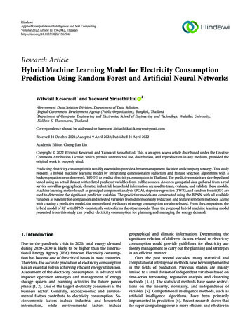
6Applied Computational Intelligence and Soft ComputingTable 2: Sampling procedures used for modeling.SampleNo. of cases and % in thesubsample10-fold cross-validationTraining619,154 cases (70%)Train: 557,238 cases (90% of learning subsample); cross-validation: 61,915 cases (10% oflearning subsample)TestTotal265,352 cases (30%)884,505 cases (100%)Table 3: The parameter structure of the BPNN predictive models.Predictive modelBPNNPCA # 1 BPNNPCA # 2 BPNNSWR BPNNRF # 1 BPNNRF # 2 BPNNNo. of nodes in input layer21913121811and SMAPE indicates greater accuracy in prediction. Thesemetrics can be formulated as follows: 1 N yt yc SMAPE 100 ,N i 1 yt yc (2) 2Ny y/N ticiRMSEi 0 .NRMSE yt max yt minyt max yt minAll parameters are explained as follows: yt is the target(real) output, yc is the calculated output, yt is an average ofthe target output, and yc is an average of the calculatedoutput and N is the total number of measurements.4. Results and Discussion4.1. Correlation and Multicollinearity Analysis. The Pearsoncorrelation coefficient (rp) is used to analyze the correlationbetween two numerical variables, and Spearman’s rankcorrelation coefficient (rs) is utilized to evaluate the correlation in categorical variables. The correlation coefficientsindicated the strength, and direction of association betweenall electricity consumption variables is shown in Figure 2.For the multicollinearity analysis, the VIF of all predictorvariables is also computed. The presence of multicollinearityimplies that the variable provides redundant informationcontained in other variables [3]. The available variables inthe modeling stage are determined by considering thecorrelation and VIF between the pair variables. Therefore,six predictor variables, namely, Electricity Substation, Season, Population N, Mean Minimum Temperature, Agriculturists, and Expenditure, are removed from the 21predictor variables. As a result, the 15 remaining predictorvariables are used as the input of SWR.4.2. Selecting Predictor Variables4.2.1. Principle Component Analysis. The 21 predictor variables are sent as the input of PCA. Since PCA works onnumerical variables, four categorical variables are convertedNo. of hidden layers322232No. of nodes in hidden layer12, 8, 28, 28, 28, 212, 8, 28, 2into numerical variables using the one-hot encoding technique. This study uses two experiments, namely, PCA # 1and PCA # 2, by using the cumulative contribution rate ofprincipal components as shown in Figure 3. For PCA # 1 andPCA # 2, the principal components with the cumulativecontribution rate reach 95% and 99%, respectively. Therefore, the first 9 and 13 principal components are consideredto be significant for PCA # 1 and PCA # 2 and used asvariables in the predictive modeling stage.4.2.2. Stepwise Regression. The 15 predictor variables fromthe correlation and multicollinearity analysis stage are usedas the input for the SWR. Since the Usage Type and TOUvariables are categorical variables, these variables are set asdummy variables to trick the SWR algorithm into correctlyanalyzing variables. Consequently, the input variables in theSWR estimation parameter consist of 22 variables. Variablesselected by SWR are summarized in Table 4, with the VIFmetrics calculated per variable. According to the VIF value,the 11 selected variables are essential in modeling theelectricity consumption. Geospatial variables are highlycorrelated with electricity consumption, among which TOUis the most important variable, followed by Usage Type.4.2.3. Random Forest. The importance of 21 predictorvariables by the RF model is listed in Table 5. From theresults, the four most important variables according to thepercentage increase in mean squared error (%IncMSE) areUsage Type, Area, Mean Station Pressure, and Industrial Labor. The variables selected by RF have two experiments: RF # 1 with 18 selected predictor variables havingimportance over 0.01 and RF # 2 with 11 variables having theimportance over 0.02.4.3. Prediction Evaluation. The results of six machinelearning models are shown in Table 6. The predictive performance is evaluated using six metrics, namely, RMSE,MAPE, NRMSE, SMAPE, R2, and Acc. The single model isdeveloped with all available 21 predictor variables (BPNN).
AreaPopulation RatioMean Station PressureMean MSL PressureMean Maximum TemperatureMean Minimum TemperatureMean Drybulb TemperatureMean Relative HumidityTotal RainfallIndustrial LaborIndustrial 1.00000.75380.0225-0.0043-0.15790.11340
predictive model for the energy cost of public buildings in Croatia.Zeki c-Suˇsacetal.[15]integratedclusteringandANN to improve the accuracy of modeling energy efficiency. Muralitharan et al. [16] proposed a convolutional neural network based optimization approach for predicting the future energy demand. P erez-Chac on et al. [17] used a big