WIXLIB

Weight Update Equation About the Optimum WeightsWeight Error Update Equationw(n 1) w(n) µ[p Rxx w(n)]Using p Rxx wow(n 1) (I µRxx )w(n) µRxx woWeight error vector: v(n) w(n) wov(n 1) (I µRxx )v(n)Matrix I µRxx must be stable for convergence ( λi 1)Assuming convergence, limn v(n) 0José Bermudez (UFSC)Adaptive FilteringIRIT - Toulouse, 201137 / 107

Convergence Conditionsv(n 1) (I µRxx )v(n);Rxxpositive definiteEigen-decomposition of RxxRxx QΛQTv(n 1) (I µQΛQT )v(n)QT v(n 1) QT v(n) µΛQT v(n)Defining ṽ(n 1) QT v(n 1)ṽ(n 1) (I µΛ)ṽ(n)José Bermudez (UFSC)Adaptive FilteringIRIT - Toulouse, 201138 / 107

Convergence Propertiesṽ(n 1) (I µΛ)ṽ(n)ṽk (n 1) (1 µλk )ṽk (n), k 1, . . . , Nṽk (n) (1 µλk )n ṽk (0)Convergence modes monotonic if0 1 µλk 1 oscillatory if 1 1 µλk 0Convergence if 1 µλk 1 0 µ José Bermudez (UFSC)Adaptive Filtering2λmaxIRIT - Toulouse, 201139 / 107

Optimal Step-Sizeṽk (n) (1 µλk )n ṽk (0); convergence modes: 1 µλkmax 1 µλk : slowest modemin 1 µλk : fastest modeJosé Bermudez (UFSC)Adaptive FilteringIRIT - Toulouse, 201140 / 107

Optimal Step-Size – continued 1 µλk 10µo1/λmax1/λminµmin max{ 1 µλk }µ1 µo λmin (1 µo λmax )µo Optimal slowest modes: ρ 1ρ 1 ;José Bermudez (UFSC)2λmax λminρ λmaxλminAdaptive FilteringIRIT - Toulouse, 201141 / 107

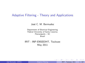
The Learning Curve – Jms(n)Excess MSENz} {XTJms (n) Jmsmin ṽ (n)Λṽ(n) Jmsmin λk ṽk2 (n)k 1Since ṽk (n) (1 µλk )n ṽk (0),Jms (n) Jmsmin NXλk (1 µλk )2n ṽk2 (0)k 1λk (1 µλk )2 0 monotonic convergenceStability limit is again 0 µ 2λmaxJms (n) converges faster than w(n)Algorithm converges faster as ρ λmax /λmin 1José Bermudez (UFSC)Adaptive FilteringIRIT - Toulouse, 201142 / 107

Simulation Resultsx(n) α x(n 1) v(n)Steepest Descent Mean Square Error0 10 10 20 20 30 30MSE (dB)MSE (dB)Steepest Descent Mean Square Error0 40 40 50 50 60 60 70020406080100120iteration140160Input: White noise (ρ 1)180200 70020406080100120iteration140160180200Input: AR(1), α 0.7 (ρ 5.7)Linear system identification - FIR with 20 coefficientsStep-size µ 0.3Noise power σv2 10 6José Bermudez (UFSC)Adaptive FilteringIRIT - Toulouse, 201143 / 107

The Newton AlgorithmSteepest descent: linear approx. of Jms about the operating pointNewton’s method: Quadratic approximation of JmsExpanding Jms (w) in Taylor’s series about w(n),Jms (w) Jms [w(n)] T Jms [w w(n)]1 [w w(n)]T H(n)[w w(n)]2Diferentiating w.r.t. w and equating to zero at w w(n 1), Jms [w(n 1)] Jms [w(n)] H[w(n)][w(n 1) w(n)] 0w(n 1) w(n) H 1 [w(n)] Jms [w(n)]José Bermudez (UFSC)Adaptive FilteringIRIT - Toulouse, 201144 / 107

The Newton Algorithm – continued Jms [w(n)] 2p 2Rxx w(n)H(w(n)) 2RxxThus, adding a step-size control,w(n 1) w(n) µR 1xx [ p Rxx w(n)]Quadratic surface conv. in one iteration for µ 1Requires the determination ofR 1xx,/Can be used to derive simpler adaptive algorithmsWhen H(n) is close to singular regularizationH̃(n) 2Rxx 2εIJosé Bermudez (UFSC)Adaptive FilteringIRIT - Toulouse, 201145 / 107

Basic Adaptive AlgorithmsJosé Bermudez (UFSC)Adaptive FilteringIRIT - Toulouse, 201146 / 107

Least Mean Squares (LMS) AlgorithmCan be interpreted in different waysEach interpretation helps understanding the algorithm behaviorSome of these interpretations are related to the steepest descentalgorithmJosé Bermudez (UFSC)Adaptive FilteringIRIT - Toulouse, 201147 / 107

LMS as a Stochastic Gradient AlgorithmSuppose we use the estimate Jms (n) E[e2 (n)] e2 (n)The estimated gradient vector becomes2ˆ ms (n) e (n) 2e(n) e(n) J w(n) w(n)Since e(n) d(n) xT (n)w(n),ˆ ms (n) 2e(n)x(n) J(stochastic gradient)and, using the steepest descent weight update equation,w(n 1) w(n) µe(n)x(n)José Bermudez (UFSC)Adaptive Filtering(LMS weight update)IRIT - Toulouse, 201148 / 107

LMS as a Stochastic Estimation Algorithm Jms (n) 2p 2Rxx w(n)Stochastic estimatorsp̂ d(n)x(n)Then,R̂xx x(n)xT (n)ˆ ms (n) 2d(n)x(n) 2x(n)xT (n)w(n) Jˆ ms (n) is the steepest descent weight update,Using Jw(n 1) w(n) µe(n)x(n)José Bermudez (UFSC)Adaptive FilteringIRIT - Toulouse, 201149 / 107

LMS – A Solution to a Local OptimizationError expressionse(n) d(n) xT (n)w(n) (a priori error)ǫ(n) d(n) xT (n)w(n 1) (a posteriori error)We want to maximize ǫ(n) e(n) with ǫ(n) e(n) ǫ(n) e(n) xT (n) w(n) w(n) w(n 1) w(n) Expressing w(n) as w(n) w(n)e(n) ǫ(n) e(n) xT (n) w(n)e(n) For max ǫ(n) e(n) w(n)in the direction of x(n)José Bermudez (UFSC)Adaptive FilteringIRIT - Toulouse, 201150 / 107

w(n) µx(n) and w(n) µx(n)e(n)andw(n 1) w(n) µe(n)x(n)Asǫ(n) e(n) xT (n) w(n) µxT (n)x(n)e(n) ǫ(n) e(n) requires 1 µxT (n)x(n) 1, or0 µ José Bermudez (UFSC)2kx(n)k2(stability region)Adaptive FilteringIRIT - Toulouse, 201151 / 107

Observations - LMS AlgorithmLMS is a noisy approximation of the steepest descent algorithmThe gradient estimate is unbiasedThe errors in the gradient estimate lead to Jmsex ( ) 6 0Vector w(n) is now randomSteepest descent properties are no longer guaranteed LMS analysis requiredThe instantaneous estimates allow tracking without redesignJosé Bermudez (UFSC)Adaptive FilteringIRIT - Toulouse, 201152 / 107

Some Research ResultsJ. C. M. Bermudez and N. J. Bershad, “A nonlinear analytical model for thequantized LMS algorithm - the arbitrary step size case,” IEEE Transactions onSignal Processing, vol.44, No. 5, pp. 1175-1183, May 1996.J. C. M. Bermudez and N. J. Bershad, “Transient and tracking performanceanalysis of the quantized LMS algorithm for time-varying system identification,”IEEE Transactions on Signal Processing, vol.44, No. 8, pp. 1990-1997, August1996.N. J. Bershad and J. C. M. Bermudez, “A nonlinear analytical model for thequantized LMS algorithm - the power-of-two step size case,” IEEE Transactions onSignal Processing, vol.44, No. 11, pp. 2895- 2900, November 1996.N. J. Bershad and J. C. M. Bermudez, “Sinusoidal interference rejection analysisof an LMS adaptive feedforward controller with a noisy periodic reference,” IEEETransactions on Signal Processing, vol.46, No. 5, pp. 1298-1313, May 1998.J. C. M. Bermudez and N. J. Bershad, “Non-Wiener behavior of the Filtered-XLMS algorithm,” IEEE Trans. on Circuits and Systems II - Analog and DigitalSignal Processing, vol.46, No. 8, pp. 1110-1114, Aug 1999.José Bermudez (UFSC)Adaptive FilteringIRIT - Toulouse, 201153 / 107

Some Research Results – continuedO. J. Tobias, J. C. M. Bermudez and N. J. Bershad, “Mean weight behavior of theFiltered-X LMS algorithm,” IEEE Transactions on Signal Processing, vol. 48, No.4, pp. 1061-1075, April 2000.M. H. Costa, J. C. M. Bermudez and N. J. Bershad, “Stochastic analysis of theLMS algorithm with a saturation nonlinearity following the adaptive filter output,”IEEE Transactions on Signal Processing, vol. 49, No. 7, pp. 1370-1387, July 2001.M. H. Costa, J. C, M. Bermudez and N. J. Bershad, “Stochastic analysis of theFiltered-X LMS algorithm in systems with nonlinear secondary paths,” IEEETransactions on Signal Processing, vol. 50, No. 6, pp. 1327-1342, June 2002.M. H. Costa, J. C. M. Bermudez and N. J. Bershad, “The performance surface infiltered nonlinear mean square estimation,” IEEE Transactions on Circuits andSystems I, vol. 50, No. 3, p. 445-447, March 2003.G. Barrault, J. C. M. Bermudez and A. Lenzi, “New Analytical Model for theFiltered-x Least Mean Squares Algorithm Verified Through Active Noise ControlExperiment,” Mechanical Systems and Signal Processing, v. 21, p. 1839-1852,2007.José Bermudez (UFSC)Adaptive FilteringIRIT - Toulouse, 201154 / 107

Some Research Results – continuedN. J. Bershad, J. C. M. Bermudez and J. Y. Tourneret, “Stochastic Analysis of theLMS Algorithm for System Identification with Subspace Inputs,” IEEE Trans. onSignal Process., v. 56, p. 1018-1027, 2008.J. C. M. Bermudez, N. J. Bershad and J. Y. Tourneret, “An Affine Combination ofTwo LMS Adaptive Filters Transient Mean-Square Analysis,” IEEE Trans. onSignal Process., v. 56, p. 1853-1864, 2008.M. H. Costa, L. R. Ximenes and J. C. M. Bermudez, “Statistical Analysis of theLMS Adaptive Algorithm Subjected to a Symmetric Dead-Zone Nonlinearity at theAdaptive Filter Output,” Signal Processing, v. 88, p. 1485-1495, 2008.M. H. Costa and J. C. M. Bermudez, “A Noise Resilient Variable Step-Size LMSAlgorithm,” Signal Processing, v. 88, no. 3, p. 733-748, March 2008.P. Honeine, C. Richard, J. C. M. Bermudez, J. Chen and H. Snoussi, “ADecentralized Approach for Nonlinear Prediction of Time Series Data in SensorNetworks,” EURASIP Journal on Wireless Communications and Networking, v.2010, p. 1-13, 2010. (KNLMS)José Bermudez (UFSC)Adaptive FilteringIRIT - Toulouse, 201155 / 107

The Normalized LMS Algorithm – NLMSMost Employed adaptive algorithm in real-time applicationsLike LMS has different interpretations (even more)Alleviates a drawback of the LMS algorithmw(n 1) w(n) µe(n)x(n) If amplitude of x(n) is large Gradient noise amplificationSub-optimal performance when σx2 varies with time (for instance,speech)José Bermudez (UFSC)Adaptive FilteringIRIT - Toulouse, 201156 / 107

NLMS – A Solution to a Local Optimization ProblemError expressionse(n) d(n) xT (n)w(n) (a priori error)ǫ(n) d(n) xT (n)w(n 1) (a posteriori error)We want to maximize ǫ(n) e(n) with ǫ(n) e(n) ǫ(n) e(n) xT (n) w(n)(A) w(n) w(n 1) w(n)For ǫ(n) e(n) we impose the restrictionǫ(n) (1 µ)e(n), 1 µ 1ǫ(n) e(n) µe(n)(B)For max ǫ(n) e(n) w(n) in the direction of x(n) w(n) kx(n)José Bermudez (UFSC)Adaptive Filtering(C)IRIT - Toulouse, 201157 / 107

Using (A), (B) and (C),k µe(n)xT (n)x(n)andw(n 1) w(n) µJosé Bermudez (UFSC)e(n)x(n)xT (n)x(n)Adaptive Filtering(NLMS weight update)IRIT - Toulouse, 201158 / 107

NLMS – Solution to a ConstrainedOptimization ProblemError sequencey(n) xT (n)w(n)(estimate of d(n))e(n) d(n) y(n) d(n) xT (n)w(n) (estimation error)Optimization (principle of minimal disturbance)Minimize k w(n)k2 kw(n 1) w(n)k2subject to:xT (n)w(n 1) d(n)This problem can be solved using the method of Lagrange multipliersJosé Bermudez (UFSC)Adaptive FilteringIRIT - Toulouse, 201159 / 107

Using Lagrange multipliers, we minimizef [w(n 1)] kw(n 1) w(n)k2 λ[d(n) xT (n)w(n 1)]Differentiating w.r.t. w(n 1) and equating the result to zero,1w(n 1) w(n) λx(n)2(*)Using this result in xT (n)w(n 1) d(n) yieldsλ 2e(n)xT (n)x(n)Using this result in (*) yieldsw(n 1) w(n) µJosé Bermudez (UFSC)Adaptive Filteringe(n)x(n)xT (n)x(n)IRIT - Toulouse, 201160 / 107

NLMS as an Orthogonalization ProcessConditions for the analysis e(n) d(n) xT (n)w(n)wo is the optimal solution (Wiener solution)d(n) xT (n)w o (no noise)v(n) w(n) wo (weight error vector)Error signale(n) d(n) xT (n)[v(n) wo ] xT (n)wo xT (n)[v(n) wo ] xT (n)v(n)José Bermudez (UFSC)Adaptive FilteringIRIT - Toulouse, 201161 / 107

e(n) xT (n)v(n)Interpretation: To minimize the error v(n) should be orthogonal to allinput vectorsRestriction: We have only one vector x(n)Iterative solution:We can subtract from v(n) its component in the direction of x(n) ateach iterationIf there are N adaptive coefficients, v(n) could be reduced to zeroafter N orthogonal input vectorsIterative projection extraction Gram-Schmidt orthogonalizationJosé Bermudez (UFSC)Adaptive FilteringIRIT - Toulouse, 201162 / 107

Recursive orthogonalizationn 0 : v(1) v(0) proj. of v(0) onto x(0)n 1:.:v(2) v(1) proj. of v(1) onto x(1).n 1 : v(n 1) v(n) proj. of v(n) onto x(n)Projection of v(n) onto x(n) Px(n) [v(n)] x(n)[xT (n)x(n)] 1 xT (n) v(n)Weight update equationscalar e(n)} {z } {zv(n 1) v(n) µ [xT (n)x(n)] 1 xT (n)v(n) x(n)e(n)x(n) v(n) µ Tx (n)x(n)José Bermudez (UFSC)Adaptive FilteringIRIT - Toulouse, 201163 / 107

NLMS has its owns problems!NLMS solves the LMS gradient error amplification problem, but .What happens if kx(n)k2 gets too small?One needs to add some regularizationw(n 1) w(n) µJosé Bermudez (UFSC)e(n)x(n)xT (n)x(n) εAdaptive Filtering(ε NLMS)IRIT - Toulouse, 201164 / 107

ε-NLMS – Stochastic Approximation ofRegularized NewtonRegularized Newton Algorithmw(n 1) w(n) µ[εI Rxx ] 1 [p Rxx w(n)]Instantaneous estimatesp̂ x(n)d(n)R̂xx x(n)xT (n)Using these estimatese(n)z} {w(n 1) w(n) µ[εI x(n)xT (n)] 1 x(n) [d(n) xT (n)w(n)]w(n 1) w(n) µ[εI x(n)xT (n)] 1 x(n)e(n)José Bermudez (UFSC)Adaptive FilteringIRIT - Toulouse, 201165 / 107

w(n 1) w(n) µ[εI x(n)xT (n)] 1 x(n)e(n)Inversion of εI x(n)xT (n) ?Matrix Inversion Formula[A BCD] 1 A 1 A 1 B[C 1 DA 1 B] 1 DA 1Thus,[εI x(n)xT (n)] 1 ε 1 I ε 2x(n)xT (n)1 ε 1 xT (n)x(n)Post-multiplying both sides by x(n) and rearranging[εI x(n)xT (n)] 1 x(n) andw(n 1) w(n) µJosé Bermudez (UFSC)Adaptive Filteringx(n)ε xT (n)x(n)e(n)x(n)xT (n)x(n) εIRIT - Toulouse, 201166 / 107

Some Research ResultsM. H. Costa and J. C. M. Bermudez, “An improved model for the normalized LMSalgorithm with Gaussian inputs and large number of coefficients,” in Proc. of the2002 IEEE International Conference on Acoustics, Speech and Signal Processing(ICASSP-2002), Orlando, Florida, pp. II- 1385-1388, May 13-17, 2002.J. C. M. Bermudez and M. H. Costa, “A Statistical Analysis of the ε-NLMS andNLMS Algorithms for Correlated Gaussian Signals,” Journal of the BrazilianTelecommunications Society, v. 20, n. 2, p. 7-13, 2005.G. Barrault, M. H. Costa, J. C. M. Bermudez and A. Lenzi, “A new analyticalmodel for the NLMS algorithm,” in Proc. 2005 IEEE International Conference onAcoustics Speech and Signal Processing (ICASSP 2005) Pennsylvania, USA, vol.IV, p. 41-44, 2005.J. C. M. Bermudez, N. J. Bershad and J.-Y. Tourneret, “An Affine Combination ofTwo NLMS Adaptive Filters - Transient Mean-Square Analysis,” In Proc.Forty-Second Asilomar Conference on Asilomar Conference on Signals, Systems &Computers, Pacific Grove, CA, USA, 2008.P. Honeine, C. Richard, J. C. M. Bermudez and H. Snoussi, “Distributedprediction of time series data with kernels and adaptive filtering techniques insensor networks,” In Proc. Forty-Second Asilomar Conference on AsilomarConference on Signals, Systems & Computers, Pacific Grove, CA, USA, 2008.José Bermudez (UFSC)Adaptive FilteringIRIT - Toulouse, 201167 / 107

The Affine Projection AlgorithmConsider the NLMS algorithm but using{x(n), x(n 1), . . . , x(n P )}Minimize k w(n)k2 kw(n 1) w(n)k2 xT (n)w(n 1) d(n) xT (n 1)w(n 1) d(n 1)subject to:. . Tx (n P )w(n 1) d(n P )José Bermudez (UFSC)Adaptive FilteringIRIT - Toulouse, 201168 / 107

Observation matrixX(n) [x(n), x(n 1), · · · , x(n P )]Desired signal vectord(n) [d(n), d(n 1), . . . , d(n P )]Error vectore(n) [e(n), e(n 1), . . . , e(n P )] d(n) X T (n)w(n)Vector of the constraint errorsec (n) d(n) X T (n)w(n 1)José Bermudez (UFSC)Adaptive FilteringIRIT - Toulouse, 201169 / 107

Using Lagrange multipliers, we minimizef [w(n 1)] kw(n 1) w(n)k2 λT [d(n) X T (n)w(n 1)]Differentiating w.r.t. w(n 1) and equating the result to zero,1w(n 1) w(n) X(n)λ2(*)Using this result in X T (n)w(n 1) d(n) yieldsλ 2[X T (n)X(n)] 1 e(n)Using this result in (*) yieldsw(n 1) w(n) µX(n)[X T (n)X(n)] 1 e(n)José Bermudez (UFSC)Adaptive FilteringIRIT - Toulouse, 201170 / 107

Affine ProjectionSolution to the Underdetermined Least-Squares ProblemWe want minimizekec (n)k2 kd(n) X T (n)w(n 1)k2where X T (n) is (P 1) N with (P 1) NThus, we look for the least-squares solution of the underdeterminedsystemX T (n)w(n 1) d(n)The solution is w(n 1) X T (n) d(n) X(n)[X T (n)X(n)] 1 d(n)Using d(n) e(n) X T (n)w(n) yieldsw(n 1) w(n) µX(n)[X T (n)X(n)] 1 e(n)José Bermudez (UFSC)Adaptive FilteringIRIT - Toulouse, 201171 / 107

Observations:Order of the AP algorithm: P 1 (P 0 NLMS)Convergence speed increases with P (but not linearly)Computational complexity increases with P (not linearly)If X T (n)X(n) is close to singular, use X T (n)X(n) εIThe scalar error of NLMS becomes a vector error in AP (except forµ 1)José Bermudez (UFSC)Adaptive FilteringIRIT - Toulouse, 201172 / 107

Affine Projection – Stochastic Approximation ofRegularized NewtonRegularized Newton Algorithmw(n 1) w(n) µ[ε̃I Rxx ] 1 [p Rxx w(n)]Estimates using time window statisticsnX11X(n)d(n)X(k)d(k) p̂ P 1P 1R̂xx 1P 1k n PnXX(k)X T (k) k n P1X(n)X T (n)P 1Using these estimates with ε̃ ε/(P 1),e(n)} {zw(n 1) w(n) µ[εI X(n)X T (n)] 1 X(n) [d(n) X T (n)w(n)]w(n 1) w(n) µ[εI X(n)X T (n)] 1 X(n)e(n)José Bermudez (UFSC)Adaptive FilteringIRIT - Toulouse, 201173 / 107

w(n 1) w(n) µ[εI X(n)X T (n)] 1 X(n)e(n)Using the Matrix Inversion Formula[εI X(n)X T (n)] 1 X(n)[εI X T (n)X(n)] 1andw(n 1) w(n) µX(n)[εI X T (n)X(n)] 1 e(n)José Bermudez (UFSC)Adaptive FilteringIRIT - Toulouse, 201174 / 107

Affine Projection Algorithm as aProjection onto an Affine SubspaceConditions for the analysis e(n) d(n) X T (n)w(n)d(n) X T (n)wo defines the optimal solution in the least-squaressensev(n) w(n) wo (weight error vector)Error vectore(n) d(n) X T (n)[v(n) w(n 1)] X T (n)w(n 1) X T (n)[v(n) w(n 1)] X T (n)v(n)José Bermudez (UFSC)Adaptive FilteringIRIT - Toulouse, 201175 / 107

e(n) X T (n)v(n

Adaptive Filter Features Adaptive filters are composed of three basic modules: Filtering strucure Determines the output of the filter given its input samples Its weights are periodically adjusted by the adaptive algorithm Can be linear or nonlinear, depending on the application Linear filters can be FIR or IIR Performance criterion Defined according to application and mathematical tractability