WIXLIB

more or less fixed, and it is determined by the outcome (thefake score) rather than the difference in score improvement.As the real test score was never realized (students who hiresomeone actually never take the exam themselves), there isreally no way to compute precisely how much the featurehas improved and put a price on it even after the fact. Theexisting model does not fit such applications.Optimal (fair) policy. The decision maker receives a truepositive (resp. false-positive) benefit (resp. penalty) u (resp.u ) when accepting a qualified (resp. unqualified) individual.Its utility, denoted by R(D, Y ), is R(1, 1) u , R(1, 0) u , R(0, 0) R(0, 1) 0. The decision maker aims to findoptimal policies for the two groups such that its expectedtotal utility E[R(D, Y )] is maximized.As mentioned earlier, there are two types of decision makers, strategic and non-strategic: A strategic decision makeranticipates strategic manipulation, has perfect information onthe manipulation cost distribution, and accounts for this indetermining policies, while a non-strategic decision makerignores manipulative behavior in determining its policies.Either type may further impose a fairness constraint C, toensure that πa and πb satisfy the following:EX PaC [πa (X)] EX PbC [πb (X)] ,(1)where PsC is some probability distribution over X associated with fairness constraint C. Many fairness notions can bewritten in this form, e.g., equal opportunity (EqOpt) (Hardt,Price, and Srebro 2016) where PsEqOpt (x) PX Y S (x 1, s),or demographic parity (DP) (Barocas, Hardt, and Narayanan2019) where PsDP (x) PX S (x s).The above leads to four types of optimal policies a decisionmaker can use, which we consider in this paper: 1) a nonstrategic policy; 2) a non-strategic fair policy; 3) a strategicpolicy; 4) a strategic fair policy. These are detailed in Sec. 3.The Stackelberg game. The interaction between the decision maker and individuals consists of the following twostages in sequence: (i) The former publishes its policies(πa , πb ), which may be strategic or non-strategic, and may ormay not satisfy a fairness constraint, and (ii) the latter, whileobserving the published policies and their realized costs, decide whether to manipulate their features.3Four types of (non-)strategic (fair) policiesNon-strategic policy. A decision maker who does not account for individuals’ strategic manipulation maximizes thebs (πs ) over Gs defined as follows:expected utility UiR hu αs PX Y S (x 1, s) u (1 αs )PX Y S (x 0, s) πs (x)dx.XDefine Gs ’s qualification profile as γs (x) PY XS (1 x, s).Then, we can show that the non-strategic policy πbsUN bargmaxπs Us (πs ) is in the form of a threshold policy, i.e., πbsUN (x) 1 γs (x) u u u(Appendix G). Throughout the paper, we will present results in the one dimensionalfeature space. Generalization to high dimensional spaces isdiscussed in Appendix B.Assumption 1. PX Y S (x 1, s), PX Y S (x 0, s) are continuous and satisfy the strict monotone likelihood ratio property,PS (x 1,s)i.e., PX Yis increasing in x R. Let unique x s beX Y S (x 0,s)such that PX Y S (x s 1, s) PX Y S (x s 0, s).Assumption 1 is relatively mild and can be satisfied bydistributions such as exponential and Gaussian, and has beenwidely used (Zhang et al. 2020; Jung et al. 2020; Barman andRathi 2020; Khalili et al. 2021; Coate and Loury 1993). Itimplies that an individual is more likely to be qualified as theirfeature value increases. Under Assumption 1, the thresholdpolicy can be written as πs (x) 1(x θs ) for some θs R.Throughout the paper, we assume Assumption 1 holds andfocus on threshold policies. We will frequently use θs todenote policy πs . Under Assumption 1, the thresholds fornon-strategic policies are characterized as follows.Lemma 1. Let (θbUN , θbUN ) be non-strategic optimal thresholds. ThenabPX Y S (θbsUN 1,s)PX Y S (θbUN 0,s)s u (1 αs )u αs .Non-strategic fair policy. Denoted as (bπaC , πbbC ), this is foundby maximizing the total utility subject to fairness constraintba (πa ) nb Ubb (πb ) suchC, i.e., (bπaC , πbbC ) argmax(πa ,πb ) na Uthat Eqn (1) holds. It can be shown that for EqOpt and DPfairness, the optimal fair policies are also threshold policiesand can be characterized by the following (Zhang et al. 2020).Lemma 2 ((Zhang et al. 2020)). Let (θbaC , θbbC ) be thresholdsin non-strategic optimal fair policies. These satisfyXs a,bnsu αs PX Y S (θbsC 1, s) u (1 αs )PX Y S (θbsC 0, s)P C (θbC )ss! 0.Strategic policy. Let p0s : PM Y S (1 0, s), the probabilitythat unqualified individuals in Gs manipulate. Under policyπs (x) 1(x θ), the decision maker’s expected utilityUs (θ) over Gs is as follows: bs (θ) u (1 αs ) FX Y S (θ 0, s) FX Y S (θ 1, s) p0Usbs (θ) is the expected utility under non-strategic policy,where URxFX Y S (x y, s) PX Y S (z y, s)dz denotes the CDF.Define manipulation benefit as s (θ) : FX Y S (θ 0, s) FX Y S (θ 1, s),representing the additional benefit an individual gainsfrom manipulation. Then, the unqualified individuals’ bestresponse (i.e., manipulation probability introduced in Sec. 2)to policy πs (x) 1(x θ) can be equivalently written asp0s (θ) : p0s (πs ) FCs ( s (θ)).The detailed derivation is in Appendix G. This manipulationprobability p0s (θ) is single-peaked with maximum occurringat x s , and limθ p0s (θ) limθ p0s (θ) 0, meaningthat when the threshold is sufficiently low or high, unqualified individuals are less likely to manipulate their features.Plugging this in the decision maker’s utility, we havebs (θ) u (1 αs ) s (θ)FC ( s (θ)) .Us (θ) Us {z}term 2: Ψs ( s (θ))(2)

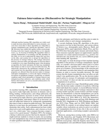
Lemma 3. For (θaUN , θbUN ), the strategic optimal thresholds,PX Y S (θsUN 1,s)PX Y S (θsUN 0,s) u (1 αs ) Ψ0s ( s (θsUN ))u αs Ψ0s ( s (θsUN )) .Strategic fair policy. Strategic fair thresholds (θaC , θbC ) arefound by maximizing the total expected utility subject to fairness constraint C, i.e., (θaC , θbC ) argmax(θa ,θb ) na Ua (θa ) nb Ub (θb ) such that Eqn. (1) holds. They can be characterizedby the following.Lemma 4. Let (θaC , θbC ) be thresholds in strategic optimalfair policies. These satisfyX PX Y S (θsC 0, s) PX Y S (θsC 1, s)Ψ0s ( s (θsC )) nsPsC (θsC )s a,bu αs PX Y S (θsC 1, s) u (1 αs )PX Y S (θsC 0, s) 0.PsC (θsC )Note that besides (θaUN , θbUN ) and (θaC , θbC ), the equations inLemmas 3 and 4 may be satisfied by other threshold pairs thatare not optimal. We discuss this further in the next section.4Impact of anticipating manipulationsImpact on the optimal policy & utility function. We firstcompare strategic policy θsUN with non-strategic policy θbsUN ,and examine how the policy and the decision maker’s expected utility differ. Let s : maxθ s (θ).Assumption 2. Ψ0s (z) is non-decreasing over [0, s ].For any threshold θ, s (θ) represents the manipulationbenefit of Gs ; those in Gs choose to manipulate if Cs s (θ). Therefore, s indicates the maximum additional benefit an individual in Gs may gain from manipulation. AsΨ0s ( s (θ)) represents the marginal manipulation gain of Gson average, Assumption 2 means that a group’s marginal manipulation gain does not decrease as manipulation benefit increases. Examples (e.g., beta/uniformly distributed cost) satisfying this assumption can be found in Appendix C. Note thatunder Assumption 2, Ψ0s (0) 0 and Ψ0s ( s (θ)) is singlepeaked with maximum occurring at x s . We assume it holdsin Sections 4 and 5. Define νs max{u αs , u (1 αs )}. Theorem 1. Let Ψ0s Ψ0s ( s ), δu u u u, and zs zs be defined such that Ψ0s ( s (zs )) Ψ0s ( s (zs )) νs .1. If αs δu , then θsUN θbsUN x s when Ψ0s νs , andθsUN {zs , zs } otherwise.2. If αs δu (resp. αs δu ), then θsUN θbsUN x s (resp.θsUN θbsUN x s ). Moreover, if Ψ0s νs , then θbsUN zs(resp. θbsUN zs ) and Us (θ) may have additional extremepoints in (zs , x s ) (resp. (x s , zs )); otherwise θbsUN is theunique extreme point of Us (θ).bs (θ) (non-strategic utility) andNote that although UΨs ( s (θ)) are single-peaked with unique extreme points,their difference Us (θ) (Eqn.(2)) may have multiple extremepoints. As we will see later, this results in strategic and nonstrategic policies having different properties in many aspects.An example of Us (θ) is shown 0.4to the right: X Y y, S s N (µy , 4.72 ), [µ0 , µ1 ] [ 5, 5], 0.2Cs Beta(10, 4), αs 0.6 andu u . The red star is the op- 0.0timal threshold θsUN zs ; two 0.2zs x s zsmagenta dots are other extremepoints of Us (θ), which are in (x s , zs ). Theorem 1 states thatUs (θ) has multiple extreme points if Ψ0s is sufficiently large,and it also specifies the range of those extreme points.Note that the maximum marginal manipulation gain Ψ0sdepends on PX Y S (x y, s), αs , and Cs . Given fixed costCs , Ψ0s increases as the maximum manipulation benefit sincreases and/or αs decreases (i.e., when there are more unqualified individuals who can manipulate). Given fixed sand αs , Ψ0s increases as cost decreases (i.e., fs (c) is shifted/skewed toward the direction of lower cost). Theorem 1shows that as compared to non-strategic policy θbsUN , strategicpolicy θsUN over(under) selects when a group is majority(un)qualified.2 In either case, as shown by Theorem 1, thismeans θbsUN is always closer to x s (the single peak of p0s (θ))compared to θsUN . Therefore, the strategic policy always disincentivizes manipulative behavior, i.e., manipulation probability p0s (θsUN ) p0s (θbsUN ).Impact on fairness. The characterization of strategic policy(θaUN , θbUN ) and non-strategic policy (θbaUN , θbbUN ) allows us tofurther compare them against a given fairness criterion C.Suppose we define the unfairness of threshold policy (θa , θb )as E C (θa , θb ) EX PaC [1(x θa )] EX PbC [1(x θb )] RθFCb (θb ) FCa (θa ), where the CDF FCs (θ) PsC (x)dx.Define the disadvantaged group under policy (θa , θb ) as thegroup with the larger FCs (θs ), i.e., the group with the smallerselection rate (DP) or the smaller true positive rate (EqOpt).Define group index s : {a, b} \ s. Note that we measureunfairness E C (θa , θb ) over the original feature distributionsPX Y S (x y, s) before manipulation.We first identify distributional conditions under which thestrategic optimal policy worsens unfairness.Theorem 2. If αs δu α s and FCs (x s ) FC s (x s ),then strategic policy (θaUN , θbUN ) has worse unfairness compared to non-strategic (θbaUN , θbbUN ), i.e., E C (θaUN , θbUN ) E C (θbaUN , θbbUN ) , C {EqOpt, DP}. Moreover, the disadvantaged group under (θaUN , θbUN ) and (θbaUN , θbbUN ) is the same.Given the conditions in Thm. 2, G s is disadvantaged under non-strategic policy. Because the majority-(un)qualifiedUs (θ)Define a function Ψs (z) : u (1 αs )FCs (z)z, then term2 in Eqn. (2) can be written as Ψs ( s (θ)), and can be interpreted as the additional loss incurred by the decision makerdue to manipulation (equivalently, the average manipulationgain by group Gs ). Further, let Ψ0s (z) be denoted as the firstorder derivative of Ψs (z), then Ψ0s ( s (θ)) indicates the decision maker’s marginal loss caused by strategic manipulation(equivalently, the marginal manipulation gain of Gs ). Thethresholds for strategic policies are characterized as follows.2We say Gs is majority-unqualified (resp. majority-qualified) ifαs δu (resp. αs δu ). When u u , a group is majority(un)qualified if more than a half of its members are (un)qualified.

group Gs (G s ) is over(under) selected under strategic policy(Theorem 1), G s becomes more disadvantaged while Gs becomes more advantaged, i.e., the unfairness gap is wider under strategic policy. Note that condition FCs (x s ) FC s (x s )holds if PX Y S (x y, a) PX Y S (x y, b). For the DP fairness measure, it holds for any distribution when αs is sufficiently large or α s sufficiently small. As shown in Sec. 7, itis also seen in the real world (e.g., FICO data).We next identify conditions on the manipulation cost, under which strategic policy (θaUN , θbUN ) can lead to a more equitable outcome or flip the (dis)advantaged group compared tonon-strategic (θbaUN , θbbUN ).UN) FCs (θbsUN ), i.e.,Theorem 3. If αa , αb δu and FC s (θb sG s is disadvantaged under non-strategic policy, then givenany G s , there always exists cost Cs for Gs such that Ψ0s issufficiently large and1. (θaUN , θbUN ) mitigates the unfairness; or2. (θaUN , θbUN ) flips the disadvantaged group from G s to Gs .Because αs δu , we have θsUN θbsUN x s (by Thm. 1).Moreover, θsUN increases as Ψ0s ( s (θ)) increases (fs (c) isskewed toward the direction of lower cost). Intuitively, asGs ’s manipulation cost decreases, more individuals can affordmanipulation; thus a strategic decision maker disincentivizesmanipulation by increasing the threshold θsUN . For any G s ,as FCs (θsUN ) increases, either the unfairness gets mitigatedUNor FCs (θsUN ) becomes larger than FC s (θ s). Proposition 1 inAppendix E considers a special case when PX Y S (x y, a) PX Y S (x y, b), and gives conditions on Ψ0s (·) under which(θaUN , θbUN ) mitigates the unfairness or flips the disadvantagedgroup when C {EqOpt, DP}.5Impact of fairness interventionsIn this section, we study how non-strategic and strategic policies are affected by fairness interventions C {DP, EqOpt}.Impact of fairness intervention on non-strategic policy.First, we consider a non-strategic decision maker and compare (θbaUN , θbbUN ) with (θbaC , θbbC ), both ignoring strategic manipulation but the latter imposing a fairness criterion. Theorem4 identifies conditions under which a fairness constrained(θbaC , θbbC ) yields higher utility from both groups comparedto unconstrained (θbaUN , θbbUN ). It is worth noting because hadstrategic manipulation been absent, (θbaUN , θbbUN ) by definitionwould attain the optimal/highest utility for decision maker.Theorem 4. Let νs max{u αs , u (1 αs )}, supposeΨ0b ( b (θbbC )) νb and Ψ0a ( a (θbaC )) νa . When FCs (θbsUN ) UN) (i.e., G s is disadvantaged under non-strategicFC s (θb soptimal policy), Ua (θbaC ) Ua (θbaUN ) and Ub (θbbC ) Ub (θbbUN )hold under any of the following cases: 1) αs δu α s ; 2)αa , αb δu and αs δu ; 3) αa , αb δu and α s δu .Condition αs , α s δu means that the qualification ratesαs , α s are sufficiently close to δu . Thm. 4 says that whenthe marginal manipulation gains of the groups under nonstrategic fair policy (θbaC , θbbC ) are sufficiently large, (θbaC , θbbC )may outperform (θbaUN , θbbUN ) in terms of both fairness and utilbs (θ) caused byity due to the misalignment of Us (θ) and Umanipulation. This means that if the decision maker lacksinformation or awareness to anticipate manipulative behavior(but which in fact exists), then it would benefit from using afairness constrained policy (θbaC , θbbC ) rather than (θbaUN , θbbUN ).Impact of fairness intervention on the strategic policy.We now compare (θaUN , θbUN ) with (θaC , θbC ). We also exploretheir respective subsequent impact on individuals’ manipulative behavior byprobabilities comparing manipulation p0a (θaUN ), p0b (θbUN ) and p0a (θaC ), p0b (θbC ) . The goal here is tounderstand whether fairness intervention can serve as incentives or disincentives for strategic manipulation. Accordingto Thm. 1, Us (θ) may have multiple extreme points understrategic manipulation if the group’s marginal manipulationgain is sufficiently large. Depending on whether Us (θ) hasmultiple extreme points, different conclusions result as outlined in Thm. 5 below, which identifies conditions underwhich fairness intervention may increase the manipulationincentive for one group while disincentivizing the other, or itmay serve as incentives for both groups.Theorem 5 (Fairness as (dis)incentives). Denote pCs : 0 UNp0s (θsC ) and pUNs : ps (θs ), we have:1. When both Ua (θ) and Ub (θ) have unique extreme points,UNCthen θsUN θsC and θ s θ smust hold. Moreover,i) If αs δu α s , then α s , κ, τ (0, 1) such thatCUNC αs κ and ns τ , we have pUNs ps , p s p s .ii) If αa , αb δu (resp. αa , αb δu ), then α s , thereexists κ (δu , 1) (resp. κ (0, δu )) such that αs CUNCκ (resp. αs κ), we have (pUNa pa )(pb pb ) 0.2. When at least one of Ua (θ), Ub (θ) has multiple extremepoints, then it is possible that s {a, b}, θsUN θsC orθsUN θsC , i.e., both groups are over/under selected underfair policies. In this case,CUNCi) If αs δu α s , then (pUNs ps )(p s p s ) 0.Cii) If αa , αb δu (or αa , αb δu ), then either pUNa pa ,CUNCUNCpUN por(p p)(p p) 0.aabbbbbs (θ)When not accounting for strategic manipulation, Uhas a unique extreme point, and imposing a fairness constraint results in one group getting under-selected and theother over-selected. In contrast, when the decision makeranticipates strategic manipulation, Us (θ) may have multiple extreme points. One consequence of this difference isthat both Ga and Gb may be over- or under-selected whenfairness is imposed, resulting in more complex incentive relationships. Specifically, if one group is majority-qualifiedwhile the other is majority-unqualified, then under-selecting(resp. over-selecting) both groups under fair policies willincrease (resp. decrease) the incentives of the former to manipulate, while disincentivizing (resp. incentivizing) the latter(by 2.(i)); if both groups are majority-(un)qualified, then thefair policy may incentivize both to manipulate (by 2.(ii)).If the marginal manipulation gain of both groups are notsufficiently large, i.e., Us (θ) has a unique extreme point,then fairness intervention always results in one group getting over-selected and the other under-selected. However,

6DiscussionIn practice, individual strategic behavior can be much morecomplicated than modeled here: those considered qualifiedmay also have an incentive to manipulate, and manipulation may only lead to partial improvement in features. Thelatter can be modeled by introducing a sequence of progressively “better” distributions (each with a different manipulation cost), and the goal of manipulation is to imitate/acquirea distributi

Fairness Interventions as (Dis)Incentives for Strategic Manipulation Xueru Zhang1, Mohammad Mahdi Khalili2, Kun Jin3, Parinaz Naghizadeh4, Mingyan Liu3 1Computer Science and Engineering, The Ohio State University 2Computer and Information Sciences, University of Delaware 3 Electrical and Computer