Transcription
BMC Ecology and Evolution(2021) 21:83Barba‑Montoya et al. BMC Ecol Evohttps://doi.org/10.1186/s12862-021-01798-6Open AccessRESEARCH ARTICLEMolecular and morphological clocksfor estimating evolutionary divergence timesJose Barba‑Montoya1,2, Qiqing Tao1,2 and Sudhir Kumar1,2,3*AbstractBackground: Matrices of morphological characters are frequently used for dating species divergence times in sys‑tematics. In some studies, morphological and molecular character data from living taxa are combined, whereas othersuse morphological characters from extinct taxa as well. We investigated whether morphological data produce timeestimates that are concordant with molecular data. If true, it will justify the use of morphological characters alongsidemolecular data in divergence time inference.Results: We systematically analyzed three empirical datasets from different species groups to test the concordanceof species divergence dates inferred using molecular and discrete morphological data from extant taxa as test cases.We found a high correlation between their divergence time estimates, despite a poor linear relationship betweenbranch lengths for morphological and molecular data mapped onto the same phylogeny. This was because nodeto-tip distances showed a much higher correlation than branch lengths due to an averaging effect over multiplebranches. We found that nodes with a large number of taxa often benefit from such averaging. However, considerablediscordance between time estimates from molecules and morphology may still occur as some intermediate nodesmay show large time differences between these two types of data.Conclusions: Our findings suggest that node- and tip-calibration approaches may be better suited for nodes withmany taxa. Nevertheless, we highlight the importance of evaluating the concordance of intrinsic time structure inmorphological and molecular data before any dating analysis using combined datasets.Keywords: Species divergence time estimation, Molecular clock, Morphological clock, Fossil calibration, BayesianinferenceBackgroundThere is a growing interest in using morphologicaldata to infer species divergence times in systematics byusing it in morphological clock analyses (e.g., [1–8]) orcombining it with molecular data in total-evidence dating approaches (e.g., [9–14]). In total-evidence dating,morphological characters from dated fossil species andextant species are analyzed along with molecular dataunder character-specific models of morphological and*Correspondence: s.kumar@temple.edu1Institute for Genomics and Evolutionary Medicine, Temple University,Philadelphia, PA 19122, USAFull list of author information is available at the end of the articlemolecular evolution (e.g., [10, 15]). Tip-calibrations aretypically used as constraints on the timing of lineagedivergence by including dated fossil species in the relaxedclock analyses [16] (Fig. 1). Moreover, in the fossilizedbirth–death (FBD) process [17, 18], the fossil species’age provides the calibration information that translatesthe morphological distances into absolute times andrates, which are propagated to the other nodes on thephylogeny.Nevertheless, utilizing morphological characters in adating analysis is complicated [11, 16, 19–23]. Morphological traits are driven by natural selection and adaptation, may experience convergent evolution, and rarelyevolve in a clock-like fashion [24, 25]. Furthermore, The Author(s) 2021. Open Access This article is licensed under a Creative Commons Attribution 4.0 International License, whichpermits use, sharing, adaptation, distribution and reproduction in any medium or format, as long as you give appropriate credit to theoriginal author(s) and the source, provide a link to the Creative Commons licence, and indicate if changes were made. The images orother third party material in this article are included in the article’s Creative Commons licence, unless indicated otherwise in a credit lineto the material. If material is not included in the article’s Creative Commons licence and your intended use is not permitted by statutoryregulation or exceeds the permitted use, you will need to obtain permission directly from the copyright holder. To view a copy of thislicence, visit http:// creat iveco mmons. org/ licen ses/ by/4. 0/. The Creative Commons Public Domain Dedication waiver (http:// creat iveco mmons. org/ publi cdoma in/ zero/1. 0/) applies to the data made available in this article, unless otherwise stated in a credit line to the data.
Barba‑Montoya et al. BMC Ecol Evo(2021) 21:83Fig. 1 Integration of morphological characters from living andextinct species in a combined analysis with molecular data. Thecombined matrices contain morphological characters from bothfossil (*) and living species, but no molecular data from fossil species.Red branch lengths are created due to the inclusion of extinct taxaand are estimated using non-molecular data. Intuitively, we expectt3, t4, and t7 to be estimated well if the non-molecular data has astrong time structure. The inclusion of non-molecular data will onlybenefit if the time structure is concordant between molecular andnon-molecular datasets. However, we emphasize the importanceof using morphological data to infer the phylogenetic position ofextinct taxa in the tree to determine which internal nodes are to becalibratedthe sampling of morphological characters is generallyfocused on taxonomically diagnostic traits. These traitsare shared by multiple lineages, with a paucity of autapomorphies and invariant characters, impacting time estimates [22]. Morphological datasets can show an extensivedifference in evolutionary rates among branches in thephylogeny, and generally, relatively smaller numbers ofmorphological characters are sampled compared to phylogenomic datasets [21].Comparisons of tip-calibration methods applying different FBD models/priors (e.g., [5, 11, 18, 19]) havereported sharp conflict between molecular, and morphological datasets under standard stochastic models causestotal-evidence dating to produce older estimates whenusing inadequate models or vague FBD priors. Furthermore, time estimates are affected by different calibration approaches that lead to different divergence timeestimates. The primary source of the problem remainsunclear, which may be investigated by examining whetherthere is significant information in the morphologicaldata to estimate divergence times (time structure). It isalso important to evaluate whether the time structure inmorphological data is concordant with the time structure in the molecular data. Such concordance will greatlyenhance the utility of total-evidence methods in whichPage 2 of 15morphological characters from extinct taxa are combined [10, 12, 13]. It also has implications for FBD datingapproaches when molecular and morphological data arejointly used [17] (Fig. 1).We have compared the intrinsic time structure offeredby morphological and molecular data with and withoutinternal node calibrations to avoid confounding the timestructure introduced by calibrations. The concordance oftime structure between morphological and molecular willbe enhanced by the presence of calibrations, which hasbeen the focus of tests by others (e.g., [5, 11, 18, 19]). Figure 1 illustrates how the phylogenetic position of a fossilspecies (D*, E*, or I*) and the time duration of the branchconnecting it to the extant tree are determined based onmorphological evidence alone in fossil tip-calibration andFBD dating approaches. The most basic requirement forreliably estimating t4 and t7 is that both morphology andmolecules produce concordant time trees. If true, theextrapolation applied in estimating t4 and t7 is appropriate because the molecular data are missing for extinctspecies. One way to evaluate this hypothesis is to assessnode ages’ concordance using the living species’ data. So,we analyzed three empirical datasets from different species groups, Hemiptera (true bugs), Hymenoptera (ants,bees, sawflies, wasps), and Spermatophyta (seed plants).Moreover, we evaluated the impact of incorporating morphological characters into a joint analysis with molecularon divergence time estimates.At the outset, we note that morphological information is often used to build evolutionary trees or placefossil taxa in the phylogeny, which usually requires a fewdiagnostic characters. However, this practice does notgenerally utilize any information on rates of evolution.Therefore, examining the concordance of intrinsic timestructure in morphological and molecular data is independently useful. Its presence is expected to produce better time estimates for the nodes created by the fossil taxaand all other nodes in the molecular tree in the combinedfossil and extant taxa analysis.ResultsMolecular versus morphological maximum likelihoodbranch lengthsThe maximum likelihood (ML) estimates of branchlengths for the same tree topology were obtained separately for molecular and morphological data. The threedatasets, Hemiptera, Hymenoptera, and Spermatophyta,showed a limited correlation and high variation betweenthe molecular and morphological branch lengths(r 0.409, 0.131, and 0.363 respectively; Fig. 2a–c). Allthree datasets showed rather short terminal morphologybased branch lengths than the molecular data, including several terminal branches of zero length. Overall, the
0.50.40.20.3Y 0.573xr 0.409p 1e 040.1Morphological treeMorphological branch lengthsMolecular treePage 3 of 15Hemipteraa(2021) 21:830.0Barba‑Montoya et al. BMC Ecol Evo0.00.50.40.30.20.10.20.30.40.5Y 1.778xr 0.363p 0.0381.01.52.0Molecular branch lengths0.5Morphological branch lengthsMorphological tree0.50.0Molecular tree0.1Spermatophytac0.4Y 0.696xr 0.131p 0.1760.00.030.30.1Morphological branch lengthsMorphological tree0.20.0Molecular treeHymenopterab0.1Molecular branch lengths0.20.070.00.51.01.52.0Molecular branch lengthsFig. 2 Branch lengths and substitution model parameters were optimized on the same topology for both molecular and morphological data onlyfor a Hemiptera, b Hymenoptera, and c Spermatophyta. The scatterplots to the trees’ right show the linear relationship between the branch lengthsobtained from molecules versus morphology. The slope, correlation coefficient (r) and p-value are shown. The black dashed line represents thebest-fit linear regression through the origin. The solid grey line represents equality between estimates0.06morphological trees had shorter terminal branch lengthsas compared to molecular phylogenies. The morphological subsets might not have sampled autapomorphies asmuch as internal branches’ changes, generating artefactually truncated terminal branches for the morphologicaltree [26]. To examine the effect of analyzing morphological data consisting only of phylogenetically informative characters, we tested for proportionality in internalbranch lengths only by excluding terminal branches. The0.3correlations improved for Hemiptera (r 0.529) andHymenoptera (r 0.622). Spermatophyta showed aweak opposite trend (r 0.028), suggesting discordanceon intermediate and deep branches (Additional file 1: Fig.S1). We also tested proportionality in branch lengths byusing a likelihood ratio test for nested models as we compared models with proportionate (linked) and unlinkedbranch lengths. For all three datasets (Hemiptera,
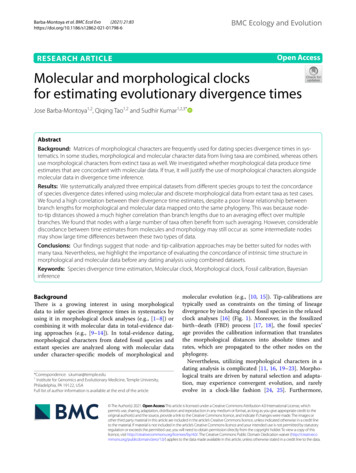
Barba‑Montoya et al. BMC Ecol Evo(2021) 21:83Hymenoptera, and Spermatophyta), unlinked modelshad significantly higher log-likelihoods (Table 1).Assessing molecular and morphological divergence timeestimatesAnalyses without internal calibrationsWe first compared time estimates applying only a rootcalibration (strategy Cr), which is critical to learn aboutthe intrinsic time structure in the data. In the Hemiptera dataset, the correlation between the time estimatesobtained from molecules and morphology was significant(R2 0.677; Fig. 3a), which was in contrast to the pattern observed for branch lengths (Fig. 2a). Overall, 72%of morphological node times fell within the 95% highest posterior density credibility intervals (HPD-CIs) formolecular node times. Some of the nodes with significantdifferences are evident in Fig. 3a and Additional file 1:Fig. S2A (nodes 56, 57, 58, 59, 60, 65, 67, 72, 73, 77, and79; numbered as in Fig. 8a). These nodes are connectedto branches that showed extreme disagreement betweenmorphological and molecular data. We found that morphological data produced wider HPD-CIs than moleculardata, the mean of %HPD-CIs (HPD-CI width/time) was111% and 89%, respectively (Fig. 4a).In the Hymenoptera dataset, the correlation betweenthe time estimates obtained from molecules and morphology was highly significant (R2 0.801), but so wasthe variation (Fig. 3d). Morphological data generally produced younger estimates than molecular data, but nodetimes were slightly older than molecular ages for a fewnodes (Fig. 3d, Additional file 1: S3A). Nodes that showa large difference in Fig. 3d and Additional file 1: Fig.S3A (nodes 57, 58, 65, 68, 72, 73, 74, 75, 76, 77, 78, 84,85, and 90; numbered as in Fig. 8b) are related to highlydisproportional branches between morphological andmolecular data. Only 62% of morphological node timesfell within the HPD-CIs for molecular time estimates(Additional file 1: Fig. S3A). Morphological data produced wider HPD-CIs than molecular data. The mean ofthe %HPD-CIs was 120% and 72%, respectively (Fig. 4b).In the Spermatophyta dataset, the correlation betweenthe time estimates obtained from molecules and morphology was again high (R2 0.844), but the linearPage 4 of 15relationship was much tighter (Fig. 3g). This is interesting because the branch lengths showed very little correspondence (see Fig. 2c). For most of the nodes in thetimetree, morphological data produced younger estimates than molecular. A likely explanation for youngermorphological time estimates than the molecular timeestimates is that terminal branches are short for morphological data due to the exclusion of singleton changes(autapomorphy) on terminal branches that result inunderestimating times near the tips of the timetree. Thenodes with the most significant differences (nodes 20,21, 28, 29, and 35; numbered as in Fig. 8c) are related tohighly discordant morphological and molecular branches(Fig. 3g, Additional file 1: Fig. S4A). 88% of morphological node times fell within the HPD-CIs for moleculartime estimates (Additional file 1: Fig. S4A). Morphological data produced wider HPD-CIs than molecular data.The mean of the %HPD-CIs was 169% and 96%, respectively (Fig. 4c).In the three datasets analyzed, the uncertainty of morphological divergence time estimates was higher thanthat from molecular data (Fig. 4a–c). The reason appearsto be because morphological characters evolve at muchmore variable rates than molecules and are sampled inrelatively smaller numbers than molecular characters,increasing the uncertainty in posterior time estimatesand, therefore, the HPD-CI widths of morphological timeestimates.Analyses with multiple calibrationsWe expected the above results to improve with theaddition of internal calibrations. So, we used multiplecalibration constraints but made them diffuse in ourfirst analyses, reflecting agnosticism on the fossil ages,which is considered a more realistic scenario (strategyC1). Indeed, in the Hemiptera dataset, the correlationbetween the time estimates obtained from moleculesand morphology became higher under this calibrationstrategy (R2 0.866; Fig. 3b). It is worth mentioningthat, although differences were still found between ageestimates from morphology and molecules, on average,timescales were similar (Fig. 3b, slope 1.103). 85% ofmorphological node times fell within the HPD-CIs forTable 1 Proportionality in morphological and molecular ML branch lengthsDatasetLinked branch lengthsUnlinked branch lengthsParametersLog-likelihood (l)ParametersLog-likelihood 3Spermatophyta95-164470.3128The model with the highest likelihood in each dataset is shown in bold type2 lp-value-37126.8471.9 0.001-69498.0916.1 0.001-164345.1250.4 0.001
30025020015010050050100Y 0.782xR 2 0.804p 2.2e 16150200250C1100Y 0.938xR 2 0.941p 5.09e–16200300C1100200300400250300C2f0100Y 0.974xR 2 0.948p 1.48e CrY 0.898xR 2 0.874p 2.2e 161501000400100300300e300Y 0.759xR 2 0.844p 3.21e 20250Y 1.021xR 2 0.901p 2.2e 160100200300400i030015050200400150b300Y 0.785xR 2 0.801p 2.2e 160Morphological timeestimates ical timeestimates (Myr)Y 1.103xR 2 0.866p 2.2e 16200250Cra0SpermatophytaPage 5 of 15200250Y 1.079xR 2 0.677p 2.2e 16(2021) 21:830HemipteraMorphological timeestimates (Myr)300Barba‑Montoya et al. BMC Ecol Evo0100200300400Molecular time estimates (Myr)Fig. 3 The posterior mean times (empty black dots) and 95% HPD-CIs under calibration strategies Cr (green lines), C1 (red lines), and C2 (purplelines) for the molecular subsets are plotted against the morphological from Hemiptera, Hymenoptera, and Spermatophyta datasets. The slope,coefficient of determination (R2) for the linear regression through the origin, and p-values are shown. The black dashed line represents the best-fitlinear regression through the origin. The solid grey line represents equality between estimatesmolecular time estimates (Additional file 1: Fig. S2B).Morphological and molecular data produced similarHPD-CIs. The mean of the %HPD-CIs from morphological data was 92% and 80% from molecular data (Fig. 4a).In the Hymenoptera dataset, the correlation betweenthe time estimates obtained from molecules and morphology remained similar (R2 0.804; Fig. 3e) than instrategy Cr. Morphological data produced younger estimates than molecular, except for a few node times, whichwere slightly older than molecular ages (Fig. 3e, Additional file 1: Fig. S3B). 42% of morphological node timesfell within the HPD-CIs for molecular time estimates(Additional file 1: Fig. S3B). Morphological data produced wider HPD-CIs than molecular data. The meanof the %HPD-CIs from morphological data was 101%and 54% from molecular data (Fig. 4b). In the Spermatophyta dataset, the correlation between the time estimatesobtained from molecules and morphology was very high
Barba‑Montoya et al. BMC Ecol Evo(2021) 21:83Page 6 of 220206040604020a0Mean percent HPD-CI widthSpermatophyta120HemipteraC2CrC1C2Calibration strategiesFig. 4 Mean relative width of 95% HPD-CIs (HPD-CI width/time) generated under calibration strategies Cr, C1, and C2 for molecular (dotted lines),morphological (dashed lines), and combined (solid line) subsets from Hemiptera (a), Hymenoptera (b) and Spermatophyta (c) datasets(R2 0.941; Fig. 3h). Morphological data produced nearlyidentical time estimates to molecular dates, except fornode 28 that was very young compared to moleculardates (Fig. 3h, Additional file 1: Fig. S4B). 94% of morphological node times fell within the HPD-CIs for moleculartime estimates (Additional file 1: Fig. S4B). Morphological data produced wider HPD-CIs than molecular data.The mean of the %HPD-CIs from morphological datawas 93% and 73% from molecular (Fig. 4c). The use ofmultiple internal calibrations reduced the uncertainty ofdivergence time estimates for both morphological andmolecular data in the three datasets (Hemiptera, Hymenoptera, and Spermatophyta), producing narrower HPDCIs than in strategy Cr.Analyses with multiple narrow calibrationsIn many studies, however, investigators apply narrowercalibration densities. So, we applied narrow calibrationconstraints in strategy C2, reflecting a prior assumptionthat fossil ages are relatively close to the "true" age of thecorresponding lineage. We thus expected an even greaterconcordance between morphological and molecular estimates of the above results when we use multiple narrowcalibrations. In effect, in the Hemiptera dataset, the concordance of dates between morphological and moleculardata became higher (R2 0.901; Fig. 3c, Additional file 1:Fig. S2C). The differences among molecular and morphological time estimates were the smallest for calibrationstrategy C2, showing a linear slope close to 1. Althoughdifferences were found between age estimates from morphology and molecules, on average, timescales were similar. Under strategy C1, 85% of morphological node timesfell within the HPD-CIs for molecular time estimates,while this proportion increased to 96% under strategy C2(Fig. 3b, c, Additional file 1: Fig. S2). Morphological andmolecular data produced similar HPD-CIs. The mean ofthe %HPD-CIs from morphological data was 70% and68% (Fig. 4a).In the Hymenoptera dataset, the concordance of datesalso improved (R2 0.874; Fig. 3f, Additional file 1: Fig.S3C). As under strategy C1, morphological data produced mostly younger estimates than molecular (withonly a few exceptions; Fig. 3f ). The differences amongmolecular and morphological time estimates were thesmallest for calibration strategy C2, showing a linearslope close to 0.9, and 69% of morphological node timesfell within the HPD-CIs for molecular time estimates(Fig. 3f, Additional file 1: Fig. S3C). Morphological dataproduced wider HPD-CIs than molecular data. The meanof the %HPD-CIs from morphological data was 93% andfrom molecular data was 52% (Fig. 4b).In the Spermatophyta dataset, the concordance of datesfrom morphological and molecular subsets remainedhigh (R2 0.948; Fig. 3i). As under strategy C1, morphological data produced nearly identical time estimatesto molecular data, except for node 28, which was veryyoung compared to molecular dates (Fig. 3i, Additionalfile 1: Fig. S4C). The differences among molecular andmorphological time estimates were the smallest for calibration strategy C2, showing a linear slope close to 1. 94%of morphological node times fell within the HPD-CIs formolecular time estimates (Fig. 3i, Additional file 1: Fig.S4C). Morphological data produced wider HPD-CIs thanmolecular data. The mean of the %HPD-CIs from morphological data was 68% and 50% from molecular data(Fig. 4c). The strong similarity between morphological
(2021) 21:83Page 7 of 15Y 0.917xR 2 0.972p 2.2e 16Cr0200300150500050100150C10100200Y 0.984xR 2 0.986p 2.2e 16C10200250300400400150200250300C2f100Y 0.987xR 2 0.985p 2.2e 16200300400300400C2200300100200300100Y 0.975xR 2 0.971p 2.2e 100100200200300Y 0.976xR 2 0.97p 2.2e 16200400200b300100C21001501000300Y 0.998xR 2 0.986p 2.2e 16200250C150Cr250400Y 0.949xR 2 0.974p 2.2e 16200300400Y 1.029xR 2 0.982p 2.2e 162002001501001003004000a500HymenopteraCombined timeestimates (Myr)Combined timeestimates (Myr)SpermatophytaDivergence time estimates from the Hemiptera combinedsubset were very similar to molecular estimates under thethree calibration strategies. However, morphological dataproduced slightly younger estimates than molecular dataunder calibration strategies Cr and C1 (Fig. 5a, b). However, under both calibration strategies, only a few nodetimes deviated from a 1:1 linear trend (Fig. 5a, b). Themean of the %HPD-CIs from the combined subset was0150Assessing divergence time estimates from combined datasets00300Cr250Y 0.974xR 2 0.962p 2.2e 1650HemipteraCombined timeestimates (Myr)250300and molecular time estimates under this calibration strategy with narrow probability densities occurs becausenodes were constrained within a restricted period forcingthe time prior and posterior estimates into an agreementso that both molecular and morphological data played aminor role in inferring divergence times [27–29]. Moreover, precise calibrations reduced the uncertainty of divergence time estimates producing narrow HPD-CIs andconcordance between morphological and molecular data.100300400i0Barba‑Montoya et al. BMC Ecol Evo0100200Molecular time estimates (Myr)Fig. 5 The posterior mean times (empty black dots) and 95% HPD-CIs under calibration strategies Cr (green lines), C1 (red lines), and C2 (purplelines) for the molecular subsets are plotted against the combined from Hemiptera, Hymenoptera, and Spermatophyta dataset using unlinked clockmodels. The slope, coefficient of determination (R2) for the linear regression through the origin, and p-values are shown. The black dashed linerepresents the best-fit linear regression through the origin. The solid grey line represents equality between estimates
Barba‑Montoya et al. BMC Ecol Evo(2021) 21:8384% under strategy Cr, 70% under C1, and 57% under C2(Fig. 4a). Under the three calibration strategies, 100% ofcombined node times fell within the HPD-CIs for molecular time estimates (Fig. 5a–c, Additional file 1: Fig. S2).Time estimates from the Hymenoptera combined subsetwere almost identical to molecular estimates under thethree calibration strategies, and only a few node timesdeviated from a 1:1 linear trend. Mainly, node 58 wasconsistently older for the molecular subset under thethree strategies. A possible reason is that the ancestraland descendant branches of node 58 have extremely different lengths in the molecular and morphological trees(Fig. 2b). This pattern persisted in the posterior time estimates. Under the three calibration strategies, 100% ofcombined node times fell within the HPD-CIs for molecular time estimates (Fig. 5d–f, Additional file 1: Fig. S3).The mean of the %HPD-CIs from the combined subsetwas 71% under strategy Cr, 54% under C1, and 50% understrategy C2 (Fig. 4b). Divergence time estimates from theSpermatophyta combined subset were nearly equal tomolecular estimates under all calibration strategies, noneof the nodes deviated from a 1:1 linear trend (Fig. 5g–i,Additional file 1: Fig. S4). The mean of the %HPD-CIsfrom the combined subset was 95% under strategy Cr,66% under C1, and 47% under C2 (Fig. 4c). Overall, combining morphological and molecular datasets had littleeffect on divergence time estimates. The strong similaritybetween combined and molecular time estimates appearsto be partly due to the relatively small morphologicaldatasets and their low information content due to variable rates [16].Bayes factor calculation for clock model selectionWe tested for proportionality in time estimates by usingthe Bayes factor to compare models with linked andunlinked relaxed-clock models [30]. Two analyses wereperformed, one using a single clock for the entire morphological and molecular dataset (linked clocks) andthe other with unlinked clocks for morphological andmolecular data [26]. To evaluate the two-clock model’sperformance, we used marginal likelihood calculation toestimate Bayes factors and posterior model probabilities.Page 8 of 15We used the stepping-stone method to obtain accuratemodel likelihoods [31].The model likelihoods are presented in Table 2. Modellikelihoods show a large difference between the two models for three datasets (Hemiptera, Hymenoptera, andSpermatophyta). The marginal likelihood estimates forthe single clock model is worse than the unlinked modelin all cases. Thus, the stepping-stone marginal likelihoodindicates strong evidence in favor of unlinked clock models for morphological and molecular data. However, timeestimates between the two clock models were almostidentical (Fig. 4, Additional file 1: Fig. S5), even thougha Bayes factor test very strongly supported the unlinkedclock model,DiscussionWhile many investigators have compared node agesestimated from morphological and molecular data, theyhave generally used multiple calibrations in their analyses(e.g., [1, 5, 8]). They often report that both data sourcesproduce comparable time estimates, but some morphological estimates have been older than their molecularcounterparts. Others have compared node age estimatesobtained from total-evidence dating involving tip dateswith those employing node-calibrations in dating [5, 10,13, 32–34]. They have reported that estimates from thetotal-evidence analysis are less sensitive to prior assumptions and tend to have smaller confidence/credibilityintervals. However, total-evidence analysis tends to produce older node age estimates, with the difference likelydue to differences in the time-prior used for node-calibration and total-evidence dating.In this study, we explored the relationship of ML estimates from the molecular and morphological branchlengths for the same phylogeny (Fig. 2a–c). We observedthat morphological evolution along the tree was generally uncoupled from molecular evolution, as the branchlength correlation was low and the dispersion high inthe three datasets analyzed (Hemiptera, Hymenoptera,and Spermatophyta). Morphological phylogenies alsodiffer from molecular phylogenies in having shorter terminal branches, a pattern that was common to all threeTable 2 Bayes factor (BF) calculation for clock-model selectionDatasetLinked clock model marginallikelihoodUnlinked clock model marginallikelihoodStepping-stone BFHemiptera Cr-37081.9-36948.1-133.7Hymenoptera Cr-69571.4-69288.3-232.1Spermatophyta Cr-164373.8-164309.4-64.4The model with the highest posterior probability in each dataset is shown in bold type
(2021) 21:83Page 9 of 15datasets. The low correlation suggests that morphological characters evolve at much more variable rates thanmolecules, and the shorter terminal branches are likelyto be due to ascertainment bias. We expected these disagreements between molecular and morphological branchlengths to have a significant detrimental impact on theefficacy of dating analysis.However, the observed concordance between divergence times produced by these two types of data seems tobe much more than that anticipated based on comparingindividual branch lengths. One fundamental reason forthis observation is that relati
Jose Barba‑Montoya1,2, Qiqing Tao 1,2 and Sudhir Kumar1,2,3* Abstract Background: Matrices of morphological characters are frequently used for dating species divergence times in sys‑ tematics. In some studies, morphological and molecular cha